
Community colleges in the United States play a critical role in promoting social mobility. This is especially the case for first-generation college students, as well as for non-traditional students and career-transitioning adults. Yet, access to equitable, high-quality two-year public colleges remains largely dependent on state- and county-level resources and economic contexts. Individuals have vastly different abilities to pay to advance their education and training, and as things stand, those with the fewest personal resources may be the ones who accrue the greatest benefit from a community college education. Furthermore, community colleges serving those with the greatest needs are likely to be situated in counties and states with the least fiscal capacity to support high-quality programs and services.
State policymakers have begun taking action on the issue of promoting equitable access to higher education with a recent push to extend free public education from the elementary and secondary level to two-year public colleges. For example, Tennessee Governor Bill Haslam approved a plan which would expand on that state’s Promise Scholarship model, which offers high school graduates tuition-free access to two-year public colleges. The planned expansion will broaden access to any Tennessee resident who does not already have a college education1. In New York, Governor Cuomo and state lawmakers reached a deal to make public two- and four-year public institutions in the state free of tuition for resident students from families with income up to $125,000.2
Importantly, the fiscal assumptions to support these plans fail to consider the ongoing costs of providing equitable access to high-quality public higher education systems, instead relying on back-of-the-envelope estimates for subsidizing existing tuition levels for expected participants. The sad fact is that, because of this, government at every level acts with very little knowledge about the actual cost of providing these systems of institutions, how to make them equitably accessible, or even, at the bare minimum, how to provide “adequate” programs and related services. Even in two-year public colleges, which focus primarily on direct instruction, the share of revenue that comes from tuition and fees is about 38 percent in New York and 42 percent in Tennessee of total current fund revenues. While the New York plan promises to maintain the existing state subsidies for higher education, it does not properly account for the real costs of providing and maintaining the system, let alone the goals and broader public interests invested in its success, relying instead solely on the existing tuition subsidy rate and prior state support.
Needless to say, providing equitable access to high quality post-secondary opportunities requires understanding the cost of providing those services. Without that knowledge, government simply cannot provide the funds and establish sustainable tax policies to cover those costs. There is and will likely always be at least some disconnect between state legislative discussions over tax policies, revenue sources, the provision of public goods and services, and the outcome quality expectations of public institutions, in that legislators will tend to (a) spend as little as feasible, holding taxes as low as possible, while (b) demanding, through accountability policies, that publicly supported institutions meet goals, standards and outcomes that far exceed the system’s capacity. This is a regrettable tendency, to be sure; but we can counter it, in the case of community colleges, by ensuring that the costs of those goals, standards, and outcomes are based on rigorous and accurate analyses, and not on hazy guesses, or on wishful thinking.
Thankfully, community college systems have well-studied analogues from which much can be learned, and adapted. In particular, scholars and policymakers working in elementary and secondary education have grappled for decades with how to implement appropriate funding mechanisms. Much like community colleges today, PreK-12 state education systems also typically operated under the “three-men-in-a-backroom” negotiation model through the early 1990s, determining state appropriations and formula distributions without any recourse to substantive calculation of costs and need. Now, however, things are very different: over the last quarter-decade, PreK-12 policy makers have introduced a number of conceptual frameworks and empirical evidence into their deliberations over state school finance policies, and their doing so has yielded significant gains in closing the gap between the amount of revenues made available to fund education, how resources are allocated, and what outcomes can reasonably be expected. In this paper, we will examine the methods that these policy makers use, and demonstrate how they can be adapted to make community college truly accessible to everyone.
Much like community colleges today, PreK-12 state education systems also typically operated under the “three-men-in-a-backroom” negotiation model through the early 1990s
Before we begin, we must acknowledge that state school finance systems remain far from perfect. Many were frozen or dismantled during the economic collapse in 2009 and haven’t been reinstated since, with their current funding remaining at levels lower than they were in 2009.3 And in other cases, state efforts to implement school finance reform were never fully implemented. For example, New York State, which recently proposed “free college” (and is one of our primary models), has yet to comply with the judicial mandate passed down in Campaign for Fiscal Equity, Inc. v State (in 2006) to adequately fund the state’s K-12 system—the standards for which have only risen in the years since.4 Further, New York has continued to ignore the state school finance formula it adopted in 2007 specifically to comply with this order, and continues to maintain one of the least equitable, and most regressive, state school finance systems in the nation.5 Similarly, Tennessee, which expanded into tuition-free community college as well, continues to have among the least adequately funded PreK-12 systems in the nation.6
But even with these setbacks and shortcomings, the focus on equity and adequacy in PreK-12 education, alongside the related conceptual and methodological developments employed by the policy makers who attend to that sector, can provide us with powerful guidance in mapping out a path toward more equitable and adequate post-secondary education systems. Preliminary analyses applying PreK-12 equity frameworks suggest that state community college systems fail to meet even the most basic equity standards: disparities in general, and instructional spending in particular, remain vast, and have not been rationally tied to variations in local economic conditions or likely student needs.
Preliminary analyses applying PreK-12 equity frameworks suggest that state community college systems fail to meet even the most basic equity standards.
These are just a taste of the revelations that the methods used in public PreK-12 systems to calculate costs have to offer. In what follows, we trace this thread of inquiry to its end, illustrating the many ways in which policy makers can apply these methods to the community college sector. In PreK-12 education, cost analyses have been used to guide the design of state school finance systems by identifying the costs of achieving state-defined outcome goals and, crucially, by distinguishing, using state aid formulas, state responsibility from local responsibility in financing those costs. Further, PreK-12 policy makers have demonstrated that cost analyses can provide insights for local institutional leaders regarding the productive and efficient allocation of resources given the specific circumstances of the student population being served. In post-secondary education, such analyses may inform both how institutions are funded through state and local resources. Further, in-depth analysis of resource allocation, program and service organization and delivery may provide guidance to institutional leaders.
Much of the hesitancy in the U.S. over providing easier and more equitable access to community college stems from a basic misunderstanding of what doing so would cost. This report recommends approaches that may be able to correct that misunderstanding, and thereby transform that hesitancy into enthusiasm. Extending these opportunities to everyone may not be as difficult, or as costly, as conventional wisdom would suggest.
Conceptions of Equity, Adequacy, and Equal Opportunity
As early as 1979, education researchers Robert Berne and Leanna Stiefel synthesized conceptual frameworks from public policy and finance, as well as evidence drawn from early litigation challenging inequities in state school finance systems, to propose a framework and series of measures for evaluating equity in state school finance systems.7 8 This seminal research laid the foundation for subsequent conceptual and empirical developments in measuring equity in PreK-12 education. Berne and Stiefel used two framing questions: (1) “Equity of what?”; and (2) “Equity for whom?” On the “what” side, Berne and Stiefel suggested that equity could be framed in terms of financial inputs to schooling, real resource inputs such as teachers and their qualifications, and, finally, outcomes. But Berne and Stiefel’s framework predated (a) judicial application of outcome standards to evaluate school finance systems, and (b) the proliferation of state outcome standards, assessments and accountability systems, first in the 1990s, and then rapidly expanding in the 2000s under the federal mandate of No Child Left Behind. The “who” side typically involved “students” and “taxpayers”—that is, a state school finance system should be based on the fair treatment of taxpayers and yield fair treatment of students.
Drawing on literature from tax policy, Berne and Stiefel (1984) adopted a definition of “fairness” which provided for both “equal treatment of equals” (horizontal equity) and “unequal treatment of unequals” (vertical equity). That is, if two taxpayers are equally situated, their tax treatment (effective rate, burden or effort) should be similar; likewise, if two students have similar needs, their access to educational programs and services or financial inputs should be similar. But, if two taxpayers are differently situated (for example, homeowner versus industrial property owner), then differential taxation might be permissible; and, if two students had substantively different educational needs, requiring different programs and services, then different financial inputs might be needed to achieve equity.
In recent decades, researchers have come to realize the shortcomings of horizontal and vertical equity delineations. First and foremost, horizontal equity itself does not preclude vertical equity, in that equal treatment of equals does not preclude the need for differentiated treatment for some (non-equals). Secondly, vertical equity requires value judgments, and then categorical determinations, as to just who is unequal, and just how unequal must their treatment be in order to be “equitable”? Federal laws (adopted in the 1970s) continue to operate into this model, applying categorical declarations as to who is eligible for differentiated treatment and frequently requiring judicial intervention to determine how much differentiation is required for legal compliance.9 But most children do not fall under the categories set forth under federal (or state) laws, even though there exist vast differences in needs across those populations of children.
An alternative, unifying approach is to suggest that the treatment, per se, is not the inputs the child receives but the outcomes that are expected of all children under state standards and accountability systems. In this sense, all children under the umbrella of these state policies are similarly situated, in that they are similarly expected to achieve the common outcome standards. Thus, the obligation of the state is to ensure that all children, regardless of their background and where they attend school, have equal opportunity to achieve those common outcome standards.
The provision of equal educational opportunity requires the differentiation of programs and services, including the provision of additional supports. This input (and process) differentiation promotes the equal treatment of similarly situated children, rather than the unequal treatment of unequals. Further, if differentiation of programs and services is required to provide students with an equal opportunity to achieve common outcomes, there exists a more viable legal equity argument on behalf of the most disadvantaged children not separately classified under federal statutes. The conception of equal opportunity to achieve common outcome goals has thus largely replaced vertical equity in the vernacular of PreK-12 equity analysis.10
The late 1980s and early 1990s saw a shift in legal strategy regarding state school finance systems away from an emphasis on achieving equal revenues across settings (neutral of property wealth) and toward identifying some benchmark for minimum educational adequacy. Politically, some advocates for this approach viewed it as infeasible for states to raise enough aid to be able to close the spending gap between the poorest and most affluent districts, meaning that achieving fiscal parity would likely require leveling down affluent districts. Focus on a minimum adequacy bar for the poorest districts would alleviate this concern, and potentially garner the political support of affluent communities, who would no longer have anything to lose.11 Koski and Reich (2006) explain that this approach is problematic, in part because minimum adequacy standards are difficult to define, and also because, when some are provided merely minimally adequate education but others provided education which far exceeds minimum adequacy, the former remain at a disadvantage. Further, the adequacy of the minimum bar is diminished by increasing that gap, because education is to a large extent a positional good, over which individuals compete, based on relative position, for access to higher education and economic prosperity.12
Others adopted a more progressive “adequacy” view, which holds that focusing on state standards and accountability systems could force legislators to provide sufficient resources for all children to meet those standards—and that state constitution education articles could be used to enforce this mandate.13 Under the more progressive alternative, equal opportunity and adequacy goals are combined: the state must provide equal opportunity for all children to achieve “adequate” educational outcomes. For this to succeed, funding must be at a sufficient overall level, and resources, programs and services must be provided to ensure that children with varied needs and backgrounds have the additional supports they need to achieve the mandated outcomes.
It remains important, however, to be able to separate equal opportunity objectives from adequacy objectives, both for legal claims and for empirical analysis. The adequacy bar can be elusive,14 and state courts are not always willing to declare that adopted assessments and outcome standards measure the state’s minimum constitutional obligation. Therefore, the state’s ability to support a specific level of “adequacy” may be subject to economic fluctuations.15 Importantly, at those times when revenues fall short of supporting high outcome standards, equal opportunity should still be preserved. That is, equal opportunity can be achieved for a standard lower than, equal to, or higher than the single “adequacy” standard.16
Critical Differences between PreK-12 and Community Colleges
There are a number of critical differences between elementary and secondary education and post-secondary education which influence both how we frame conceptions of equity, equal opportunity, and adequacy, as well as how we approach cost estimation. First, post-secondary education is not compulsory, and so does not generally enjoy state constitutional protection in the way that elementary and secondary education do. Second, because post-secondary education is largely considered a personal choice, and there exist many choices for academic and career paths within that choice set, there are no obvious common outcome goals for post-secondary education.
When evaluating the adequacy of elementary and secondary education systems, state courts often reference the importance of distal outcomes such as “knowledge of economic, social, and political systems to enable the students to make informed choices” or “sufficient training or preparation for advanced training in either academic or vocational fields so as to enable each child to choose and pursue life work intelligently.”17 However, a convenient fallback, and increasingly prevalent standard, for elementary and secondary education is that graduates of a state’s secondary schools should be sufficiently prepared for the next stage of their education—or to be “college or career ready.” “College readiness” is often reduced to measures of course completion (sometimes with standardized end-of-course assessments), graduation, and scores on those standardized tests presumed predictive of success in introductory college-level coursework.18
Outcome expectations for post-secondary education are notably more complex, more difficult to measure and more varied across individuals and institutions, especially where terminal degrees or certificates are involved. There exist few standardized end-of-course assessments, though professional licensure exams are required in some fields. Most importantly, as noted above, students choose widely varied career paths, from culinary training to nursing to air traffic control. Demand for graduates in these fields varies over time and across regions, as do wages, rendering the establishment of common economic outcome measures problematic. Finally, for many public two-year colleges, the dominant outcome is matriculation to four-year colleges, which requires yet another unique set of considerations.
Another difference is the assumption that elementary and secondary education must more comprehensively cover the costs associated with equitable access to adequate programs and services. This often includes the provision of transportation, as well as materials, supplies and equipment. Equity and adequacy are compromised when those costs are passed along to students and their families. In many states it is impermissible to charge students to be transported to school or to purchase their own textbooks, as these are necessary elements of the state’s constitutional obligation.
From Conceptions to Costs
In this section we explain how to transition from conceptions of equity, equal educational opportunity, and educational adequacy to the considerations required for accurately estimating the costs of achieving these goals. Perhaps most importantly, estimation of “cost” requires some outcome goal, or some measure of the quality of the product and/or service in question.19 That is, in performing cost estimation, the researcher must necessarily ask, “the cost of what?” This is entirely consistent with our framing of equal educational opportunity, which asks whether all children have an equal opportunity to achieve some specified set of outcome goals. Thus, the point here is to determine the “costs” associated with achieving the outcome goals in question, and whether and how those “costs” vary across children and settings.
In this section, we begin with a discussion of the complexities associated with setting outcome goals, and how outcome goal-setting may differ in post-secondary education when compared with the goal-setting done for elementary and secondary education systems. Next, we explore (a) cost factors and (b) risk factors, which research on elementary and secondary school systems have shown to collectively affect the “costs” of achieving common outcome goals. Finally, discuss similar types of factors that might affect the cost of providing an equal educational opportunity in the context of post-secondary education.
Toward What Common Outcomes
Moving from conceptions of equal educational opportunity and adequacy to the application of cost estimation requires taking broadly framed outcome goals and reducing them to measures and indicators. In elementary and secondary education, broad outcome declarations, judicial or legislative, such as providing for a “meaningful high school education” or ensuring that all children are “college and career ready,” must be operationalized into more practical, tangible measures and indicators. Furthermore, in order to estimate equal educational opportunities, common outcome measures must be established—that is, what common outcome are all students expected to have equal opportunity to achieve? As noted above, most states have adopted standards and measures of accountability that they apply across all of their elementary and secondary school systems. In some cases, state courts have used these standards and measures as the basis for determining broader constitutional requirements.
Elementary and secondary education standards and accountability systems tend to be based primarily on (a) standardized assessments of reading and math from grades 3 to 8, and sometimes 10 and/or 11, and (b) other measures, such as four-year graduation rates. Standardized assessments often have assigned “cut-scores” that declare whether each student’s performance is “proficient” (meeting basic standards) or not, and in some states, students must pass a common high school exam in order to receive a diploma. Increasingly, states have also adopted measures of test score growth, and in some cases test score growth conditional on risk factors (comparing students of similar backgrounds and needs).20 These systems of measures and indicators, though limited, often serve to provide convenient benchmarks for judicial analysis and for empirical estimation of “costs.”21
Analyses of elementary and secondary education system outcomes often look at system outcomes as a whole—school district outcomes—presuming that a primary goal for all (or at least most) students is post-secondary access, and perhaps more specifically, preparation to undertake traditional undergraduate general education coursework. That is, we often conveniently ignore the role of vocational programs and specialized magnet secondary schools by focusing on a hypothetical “general education” majority. Rarely if ever have elementary and secondary cost analyses considered whether the arts magnet high school is providing equitable, adequate specialized training for students to productively contribute as creative artists, or whether vocational programs are achieving a sufficient percentage of job placements that result in livable wages. Recent emphasis on “common core standards” and “college and career readiness” for all students has pushed specialized alternatives further to the margins of secondary schooling.22
Rarely if ever have elementary and secondary cost analyses considered whether the arts magnet high school is providing equitable, adequate specialized training for students to productively contribute as creative artists, or whether vocational programs are achieving a sufficient percentage of job placements that result in livable wages.
As noted above, post-secondary education, unlike elementary and secondary education, is not compulsory for all students, though there is increased interest in ensuring that it is accessible to all students. As we move the conversation from elementary and secondary to post-secondary education systems, we can no-longer sidestep issues of student choice and specialization. While economic outcomes have some influence on how students choose their courses and programs, they remain secondary to “beliefs about course enjoyment and grades.”23 This complicates our options for outcome measures, since the outcomes of uncommon choices and aspirations made by students in post-secondary education vary. However, the logic behind the “general education” outcome orientation in elementary and secondary education is that providing equal opportunity to access and success in post-secondary education will provide students more equitable access to economic and civic participation in modern society. That is, it is presumed that having a “meaningful high school education,”24 for example, prepares one to attend and complete college, which is increasingly necessary for achieving gainful employment in a modern economy.
Our primary interest in this paper is the translation of cost analysis approaches from elementary and secondary education to two-year public colleges, or community colleges. In some cases, two-year degrees are terminal degrees leading directly to professional careers, and in other cases, two-year colleges serve in a transitional role to four-year degrees. Many students make the transition to four-year colleges before even completing the two-year degree. A recent report from the National Student Clearinghouse described the following three major patterns for students attending community colleges:
- College Persistence: Six out of ten students who begin college at a two-year public institution persist into the second fall term. Of the students who persist, nearly one in five do so at a transfer destination.
- Transfer and Mobility: Of all students who began college at two-year public institutions in fall 2008, 24.4 percent transferred to a four-year institution within six years and 15 percent transferred to two-year institutions (lateral transfer), for an overall transfer rate of 39.6 percent.
- Certificate and Degree Completion: In the 2016 Signature Report on completion rates, the National Student Clearinghouse Research Center found that 30 percent of the fall 2010 entering cohort of community college students completed their first credential within six years at either the initial institution where they were enrolled or at a different two-year college. In addition, another 9.3 percent completed their first credential at a four-year institution.25
That is, for nearly 40 percent of community college students, the eventual outcome is not degree completion and employment but rather transfer to another institution. Community college for many is yet another intermediate step. Further, a related NSC report explained:
- One in ten students who started in two-year public institutions transferred and graduated from a four-year institution without receiving any credential from their starting institution.
- Traditional graduation-rate measures that focus only on completions at the starting institution do not account for this type of outcome, even though it is a well-worn pathway pathway that has been increasing in both incidence and attention in today’s resource-constrained policy environment.26
Several authors have estimated the long term economic value (distal outcomes) of these shorter term (proximal) outcomes: persistence and completion. For example, several studies find that the completion of associate’s degrees leads to positive increases in wages in almost every field, but that the increases vary widely by field.27 Others have found that certificate completion also leads to economic benefits, but that those benefits tend to be smaller than the benefits for degree completion.28 More specifically, “the return to credits in many career and technical education (CTE) subfields is significant, positive, and oftentimes strong, while the reverse is true of credits in many non-CTE subfields.”29
So, as with secondary education, we know that the intermediate outcomes of completion alone are significant. But, the choices of programs, and even of individual courses within programs, strongly influence eventual earnings.30 Thus, while it might be desirable to find some measures of gainful employment or wages (distal outcomes), it may be more practical to focus initial efforts on studying costs in community colleges in relation to the proximal outcomes—persistence and completion—which are associated with those longer term benefits.
On a related note, Bahr explains that the collective choices of students, given local and regional context, can shape the overall mission of community colleges. Bahr describes five types of community colleges: Community Education Intensive, Transfer Intensive, Workforce Development Intensive, High-Risk Intensive, and Mixed Use.31 These categories are derived from student behavioral profiles for first-time attendees, identified as drop-in, experimental, noncredit, terminal vocational, transfer, and exploratory. Bahr then investigates “whether the patterns of student use that characterize the five types appear to be primarily a consequence of institutional policies and practices or, conversely, a product of localized community demand and the associated circumstances and choices of the students who attend a given college.” Bahr finds that “variation in patterns of student use across institutions appears to be primarily a product of localized community demand,” and that “institutions that differ in terms of dominant or disproportionate patterns of student use also differ significantly and systematically on a number of measures of institutional performance.”32 Mixed Use community colleges are relatively balanced in their student profiles; Community Education Intensive institutions are represented by high concentrations of drop-in and non-credit students; Transfer Intensive institutions by high rates of transfer and exploratory students; Workforce Development by high rates of terminal vocational profiles; and High-Risk Intensive by high rates of experimental profiles and relatively low rates of transfer profiles, where students of historically disadvantaged backgrounds are disproportionately represented among experimental profiles. Bahr’s typology and methods might prove useful for classifying community college types for purposes of comparing costs, where students’ collective goals and institutional contexts share similarities.
Cost and Risk Factors
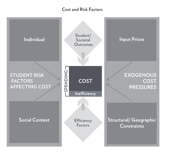
Equal opportunity requires that students, regardless of their personal and educational backgrounds, have equalized chances to succeed on the proximal or distal outcomes in question. Two broad categories of factors affect the “costs” of providing equal educational opportunity: (1) cost factors, i.e. input price levels and other geographic pressures, and (2) risk factors, i.e. characteristics related to individual or collective student needs.33 One view of educational equity—which falls short of equal opportunity—is that all students should be provided not merely with equal dollar inputs to their schooling but with equitable real resources. The “real resources” of schooling are the people (human resources including faculty and staff), space (capital assets), and the materials, supplies and equipment that go into the provision of educational services (direct instruction and all related supports). Real resource equity is affected by input price variation and by other geographic cost pressures. In contrast, student background characteristics affect the extent to which real resources—programs and services—must be differentiated in order to provide students with equal opportunity to achieve outcome goals.
One view of educational equity—which falls short of equal opportunity—is that all students should be provided not merely with equal dollar inputs to their schooling but with equitable real resources.
Figure 1 lays out the relationship between cost pressures, risk factors and outcome goals, as realized through institutional spending on program and service delivery. The amount that must be spent by an institution toward achieving some common outcome goals depends on these cost factors and on student characteristics. An important additional feature of this figure is the delineation between spending and cost. Institutions might spend on things not directly associated with achieving the measured outcomes. That is, an institution might spend more than it would cost at a minimum to achieve the desired outcomes given existing cost pressures and risk factors. That margin of spending above cost might be characterized as “inefficiency,” but in this case, “inefficiency” takes on a broad meaning, including spending on programs and services which may be valued but not measured as primary goals/objectives. For example, institutional expenditures may include expenditures on community-based programs and events, such as athletics and the arts, which may marginally, if at all, contribute to student persistence and completions. This is not to suggest, however, that these expenditures are unnecessary or inappropriate. Rather, they are simply not captured by the outcomes being measured because they serve a different, but still valuable, purpose.
Figure 1.
Providing equitable real resources across all locations in a system requires addressing differences in the prices of those resources from one location to another, as well as other potential geographic and structural constraints on delivering those resources. For example, recruiting and retaining faculty of comparable qualifications may require different wages in Garden City, Kansas when compared with Kansas City, Kansas. Similarly, the prices of construction, utilities and other materials, supplies, and equipment may differ. These are what we call “input price” differences. Most studies of elementary and secondary education costs focus on variation in the competitive wages of teachers, usually by comparing teacher wages to those of similarly educated, same-age workers in the same labor market.34
Providing equitable real resources across all locations in a system requires addressing differences in the prices of those resources from one location to another, as well as other potential geographic and structural constraints.
Other geographic factors might also affect the costs of providing comparable programs and services. For example, to provide a comparable array of program options in a low-population area may mean having fewer students enrolled in some programs, leading to higher per-pupil costs.35 Rural secondary schools face a similar constraint with respect to the provision of advanced courses, and even rural elementary schools may be required to operate suboptimal class sizes. These costs, to the extent that they are by necessity rather than choice (i.e., the choice to operate a small school in a population-dense area), should be considered in cost estimation and aid formulas. Transportation costs are also affected by the relative sparsity of student populations, and are necessary to address to ensure equitable access.
The upper portion of Table 1 lists price pressures and geographic cost factors commonly cited in elementary and secondary education cost analyses alongside potential cost factors for consideration in post-secondary cost analysis. In elementary and secondary education, two approaches have been taken to address variation in teacher wages. In the first, the comparable wage index approach, the goal, as noted above, is to index the variation in wages across labor markets for individual in non-teaching professions who have similar education levels (and similar ages) to those working in teaching professions. The premise behind this approach is that to the extent that non-teaching wages vary from one labor market to the next, so too will teacher wages have to vary in order to remain similarly competitive (whether equal or not to non-teacher wages). Similar approaches are clearly applicable for community college faculty.
The alternative sometimes applied in elementary and secondary education analysis is to attempt a more fine-grained indexing that additionally takes into account localized working conditions and preferences, in order to level the playing field for teacher recruitment and retention across local districts within labor markets. This approach—the hedonic wage model36—faces the challenge of precisely identifying those compensating differentials, or the higher compensation rates required to hire and retain staff in staff roles and settings that are perceived to be more demanding and/or less pleasant.37 This approach may also be less applicable to community colleges, as it is less likely that there are, or will be, several community colleges operating within a single labor market, competing for the same pool of potential faculty.
Analyses of elementary and secondary education costs also typically include measures of total enrollment size, indicators of grade ranges served, and, in some cases, indicators of specialized programming. Similar issues may be applicable to community colleges, where Bahr’s typology mentioned above may prove useful for institutional type classification.
| Table 1. Cost and Risk Factors | |||
| Factors | Pre-K through 12 | Community College | |
| Input Price Pressures (to achieve real resource equity) | Personnel and Non-Personnel | Macro (labor market entrants): Comparative Wage Index38 Micro (sorting across jurisdictions/schools): Hedonic Wage Model39 |
Wages40 |
| Geographic Structural Constraints (to achieve real resource equity) | Economies of scale41 Grade ranges42 Specialized programs/schools Capital stock43 |
Scale44 Program type45 |
|
| Risk Factors & Costs of Risk Mitigation (to achieve equal educational opportunity) | Collective/ Population | Poverty46 Persistent poverty47 (Poverty density) Race48 |
Family income First-generation Academic preparation49 (course rigor, peer composition) |
| Individual | Language proficiency50 Disability51 |
||
For student risk factors, the idea is that certain measurable attributes of individual students, or collectively of the population served by an institution, may be predictive of outcomes, including risk of failure on the outcomes selected for measurement. Further, it is assumed that appropriate interventions—which come with additional costs—can mitigate these risks. Table 1 lists commonly cited risk factors from elementary and secondary education cost analysis, as well as potential risk factors based on research on post-secondary education outcomes. Analyses of the costs of achieving common outcome goals in elementary and secondary education use a variety of poverty and socioeconomic indices to characterize the student populations served by schools and districts. Measures of poverty and socioeconomic status measures serve to broadly characterize risk and capture the costs associated with schoolwide strategies thought to mitigate those risks, including provision of smaller class sizes, early childhood programs, and the need for compensating differentials for teacher recruitment and retention, to name a few. Cost analyses in elementary and secondary education also commonly include measures of the proportions of the student population with disabilities (preferably by severity of disabilities), and of those who are English-language learners. These “risk” factors are associated with specific program and resource interventions for the targeted student population, whereby the premise is that these interventions are necessary to provide equal opportunity to succeed on the common outcome goals.
Literature on community college outcomes—typically measured as intermediate outcomes of persistence and completion—addresses similar factors. Family income, generational status,52 “non-traditional” (adult) learners, and prior academic preparation each play a role in the preparedness of students to persist and complete their programs of study, and in the types of services, supports and modifications to instructional programs and courses that might improve persistence and completion rates for high-risk students. Language barriers and disability status, and other possible factors, including whether a student is an adult learner, likely also warrant consideration.53
The problem of under-preparedness—and lack of rigorous secondary curricular options—raises a systemwide concern.
The problem of under-preparedness—and lack of rigorous secondary curricular options—raises a systemwide concern (PreK-16). Taking community colleges as independent of elementary and secondary education, under-preparedness is a “cost factor” outside of the control of community colleges. Similarly, the under-preparedness of three- and four-year olds is a risk and cost factor for elementary schools. Under-preparedness for college is controllable (not exogenous) within the larger system, however, and should be addressed earlier in the pipeline, with sufficient resources targeted according to student backgrounds and needs. This is especially true of the types of disparities in preparedness identified by Flores and colleagues, where graduates of predominantly minority high schools had less access to advanced coursework.54 That is, the inequities of the elementary and secondary system disproportionately affect high-risk students, the additional costs of which are passed on to the post-secondary education level.
Methods of Cost Estimation
The purpose of this paper is to consider methods used in cost estimation at the PreK-12 schooling level in order to establish a framework that will allow us to estimate the costs of achieving some common set of outcome goals for students in community college. This section will specifically explore the frameworks necessary to estimate the costs of providing equal opportunity to community college students to achieve a common set of outcome goals, regardless of students’ personal backgrounds or where they attend. As noted in the previous section, this discussion requires identifying and accounting for the various “risk” and “cost” factors that mediate the relationship between institutional resources and student outcomes.
In this section, we summarize and classify methods used for the estimation of costs for elementary and secondary schools. Specifically, we focus on methods used in recent decades for determining the costs of meeting state standards, where the findings yielded by these methods have often informed either judicial deliberations over the adequacy of state public elementary and secondary school finance systems, or legislative deliberations regarding appropriate reforms to those systems, or both.
Frameworks from PreK-12
Cost estimation applied to elementary and secondary education has typically fallen into two categories:
- Input-oriented analyses identify the staffing, materials, supplies and equipment, physical space, and other elements required to provide specific educational programs and services. Those programs and services may be identified as typically yielding certain educational outcomes for specific student populations when applied in certain settings.
- Outcome-oriented analyses start with measuring student outcomes as generated by the specific programs and services offered by institutions. They can then explore either the aggregate spending on those programs and services that yield specific outcomes, or explore in greater depth the allocation of spending on specific inputs.
The primary methodological distinction here is whether one starts from an input perspective or from one that designates specific outcome measures. One approach works forward, toward actual or desired outcomes, starting with inputs; the other backwards, from outcomes achieved. Ideally, both work in concert, providing iterative feedback to one another. Regardless, any measure of “cost” must consider the outcomes to be achieved through any given level of expenditure and resource allocation.
Input-Oriented Cost Analysis: Setting aside for the moment the modern proprietary jargon of costing-out studies, there really exists just one basic method for input-oriented analysis, which since the late 1970s has been given two names: the Ingredients Method and Resource Cost Modeling (RCM); we will refer to it as the latter. RCM involves three basic steps:
- Identifying the various resources, or “ingredients,” necessary to implement a set of educational programs and services (where an entire school or district, or statewide system for that matter, would be a comprehensive package of programs and services);
- Determining the input price for those ingredients or resources (considering competitive wages, other market prices, etc.); and
- Combining the necessary resource quantities with their corresponding prices to calculate a total cost estimate (Resource Quantities × Price = Cost).
Resource cost modeling was applied by Jay Chambers and colleagues in both Illinois and Alaska in the early 1980s to determine the statewide costs of providing the desired (implicitly “adequate”) level of programs and services, long before its use in the context of school finance adequacy litigation in Wyoming in 1995.
A distinction between the input-oriented studies conducted prior to modern emphasis on outcome standards and assessments is that those studies focused on tallying the resource needs of education systems designed to provide a set of curricular requirements, programs and services intended to be available to all children. Modern analyses instead begin with goals statements—or the outcomes the system is intended to achieve—and then require consultants and/or expert panels to identify the inputs needed to achieve those goals. Nonetheless, the empirical method is still one of tallying inputs, attaching prices and summing costs.
RCM can be used to evaluate:
- Resources currently allocated to actual programs and services (geared toward measurably achieving specific outcomes);
- Resources needed for providing specific programs and services where they are not currently being provided; and
- Resources hypothetically needed to achieve some specific set of outcome goals—as defined by both depth and breadth.
In the first case, where actual existing resources are involved, one must thoroughly quantify those inputs, determine their prices, and sum their costs. If seeking findings that are generalizable, one must explore how input prices (from teacher wages to pencils and paper) vary across the sites where the programs and services are implemented, and whether context (economies of scale, grade ranges) affects how inputs are organized in ways consequential to cost estimates.
In the second case, where hypothetical (or not-yet-existing) outcome goals are involved, a number of approaches can be taken—including organizing panels of informed constituents, including professionals and researchers—to hypothesize the resource requirements for achieving desired outcomes with specific populations of children educated in particular settings. Competing consultants have attached names including Professional Judgment (PJ) and Evidence-Based (EB) to the methods they prefer for identifying the quantities of resources or ingredients. Professional Judgment involves convening focus groups to propose resource quantities for hypothetical schools defined by varying levels of school needs, scale of operations, and geographic setting to achieve specific outcomes, while Evidence-Based methods involve the compilation of published research into model schools presumed adequate regardless of context because of their reliance on published research where the findings are assumed to be externally generalizable.
One should expect a well-designed input-oriented resource cost analysis to engage informed constituents in a context-specific process that also makes available sufficient information (perhaps through prompts and advanced reading) on related “evidence.” Put bluntly, these two methods should not be applied exclusively in isolation from one another. Even under the best application, the result of this process is a hypothesis of the resource needs required to fulfill the desired outcome goals. Where RCM is applied to programs and services already associated with certain actual, measured outcomes, that hypothesis is certainly more informed, though not yet formally tested in alternative settings.
Outcome-Oriented Cost Analysis: The primary tool of outcome-oriented cost analysis is the Education Cost Function (ECF).55 Cost functions typically focus on the outcome-producing organizational unit, or decision making unit (DMU) as a whole—in this case, schools or districts—evaluating the relationship between aggregate spending and outcomes, given the conditions under which the outcomes are produced. The conditions regularly include economies of scale (higher unit production costs of very small organizational units), variations in labor costs, and, in the case of education, characteristics of the student populations which may require greater or fewer resources to achieve common outcome goals.
Identifying statistical relationships between resources and outcomes under varied conditions requires high-quality and sufficiently broad measures of desired outcomes, inputs, and conditions, as well as a sufficient number of organizational units that exhibit sufficient variation in the conditions under which they operate. Much can be learned from the variation that presently exists across our local public, charter, and private schools regarding the production of student outcomes, the aggregate spending, and the specific programs and services associated with those outcomes.
That said, cost functions have often been used in educational adequacy analysis as a seemingly black-box tool for projecting the required spending targets associated with certain educational outcomes. Such an approach provides no useful insights into how resources (staffing, programs and services, etc.) are organized within schools and districts at those spending levels and achieving those targets. We argue that this is an unfortunate, reductionist use of the method.
As an alternative to the black-box spending prediction approach, cost functions can be useful for exploring how otherwise similar schools or districts achieve different outcomes with the same level of spending, or the same outcomes with different levels of spending. That is, there exist differences in relative efficiency. Researchers have come to learn that inefficiency found in an ECF context is not exclusively a function of mismanagement and waste, and is often statistically explainable. Inefficient “spending” in a cost function is that portion of spending variation across schools or districts that is not associated with variation in the student outcomes being investigated, after controlling for other factors. The appearance of inefficiency might simply reflect the fact that there have been investments made that, while improving the quality of educational offerings, may not have a measurable impact on the limited outcomes under investigation. It might, for example, have been spent to expand the school’s music program, which may be desirable to local constituents. These programs and services may affect other important student outcomes including persistence and completion, and college access, and may even indirectly affect the measured outcomes.
As an alternative to the black-box spending prediction approach, cost functions can be useful for exploring how otherwise similar schools or districts achieve different outcomes with the same level of spending, or the same outcomes with different levels of spending.
Factors that contribute to this type of measured “inefficiency” are also increasingly well-understood, and include two general categories: fiscal capacity factors and public monitoring factors.56 For one, local public school districts with greater fiscal capacity—that is, those with a greater ability to raise funds, and who spend more—are more likely to do so, and may spend more in ways that do not directly affect measured student outcomes. But that is not to suggest that all additional spending is frivolous, especially where outcome measurement is limited to basic reading and math achievement. Public monitoring factors often include such measures as the share of school funding coming from state or federal sources, where higher shares of intergovernmental aid are often related to reduced local public involvement (and monitoring).
A thorough ECF model considers spending as a function of (a) measured outcomes, (b) student population characteristics, (c) characteristics of the educational setting (economies of scale, population sparsity, etc.), (d) regional variation in the prices of inputs (such as teacher wages), (e) factors affecting spending that are unassociated with outcomes (“inefficiency” per se), and (f) interactions among all of the above.
Comparing Input and Outcome Methods: Table 1 summarizes our perspectives on education cost analysis as applied to measuring educational adequacy and organizes the methods into input-oriented and outcome-oriented methods, which are subsequently applied to hypothetical or actual spending and outcomes. The third column addresses the method by which information is commonly gathered, such as focus groups, or consultant synthesis of literature. The fourth column adds another dimension: the unit of analysis, which also includes the issue of sampling density. Most focus group activities can only practically address the needs of a limited number of prototypical schools and student populations, whereas cost modeling involves all schools and districts, potentially over multiple years (to capture time dynamics of the system in addition to cross-sectional variation). It can be difficult to fully capture the nuanced differences in cost factors affecting schools and districts across a large, diverse state through only four to six (or even forty) prototypes. Alternatively, one might hybridize traditional PJ approaches with survey techniques to gather information across a wider array of settings, thereby increasing the sampling density).57
| Table 2. Approaches to Input and Outcome Oriented Cost Analysis | |||||
| General Method | Outcome/ Goal Basis |
Information Gathering | Unit of Application | Strengths | Weaknesses |
| Input-Oriented (Ingredients Method or Resource Cost Model) | Hypothetical | Focus Groups (Professional Judgment) | Prototypes (limited set) | Stakeholder involvement.
Context sensitive. |
Only hypothetical connection to outcomes.
Addresses only limited conditions/settings. |
| Hypothetical | Consultant Synthesis (Evidence Based) | Single model (applied across settings) | Limited effort. Ability to use and apply one-size-fits-all model to any situation.
Built on empirically validated strategies. |
Aggregation of “strategies” to whole school is suspect.
Transferability of effective strategies is limited. Not context-sensitive. |
|
| Actual | State data systems that contain school-level information: personnel data, annual financial reports, outcome measures. | Schools/districts sampled from outcome-based modeling (efficient producers of outcomes under varied conditions) | Grounded in reality (what various schools/districts actually accomplish and how they organize resources) | Requires rich personnel, fiscal, and outcome data.
Potentially infeasible where outcome goal far exceeds actual observed outcomes. |
|
| Outcome-Oriented (Cost Function) | Actual | State fiscal data systems that provide accurate district- or school-level spending estimates, including district spending on overhead. | All districts/schools over multiple years. | Based on estimated statistical relationship between actual outcomes and actual spending.
Evaluates distribution across all districts/schools. |
Requires rich, high-quality data on personnel, finances and, outcomes.
Focuses on limited measured outcomes. Limited insights into the internal resource use/allocation underlying the cost estimate. |
While all methods have strengths and weaknesses, some of the weaknesses represent critical flaws. For example, where the objective is to determine comprehensive, institutional costs of meeting specific outcome goals across varied contexts, the evidentiary basis for “evidence-based” analyses may fall short. While research evidence can be useful for identifying specific interventions which may yield positive outcomes, research evidence rarely addresses whole institutions or provides evidence on a sufficient array of interventions, which, if cobbled together, could constitute an entire institution (inclusive of administrative structures, etc.).58
The greatest shortcoming of the arguably more robust RCM process used in Professional Judgment is that the link between resources and outcomes is hypothetical (i.e., based solely on professional opinion). The greatest weaknesses of cost modeling are (a) that predictions may understate true costs of comprehensive adequacy where outcome measures are too narrow, and (b) that like any costing-out method, when desired goals far exceed those presently achieved, extrapolations may be suspect. Stressing the latter point, cost modeling and other approaches to costing out are most useful where there exist institutions in the sample or population which actually perform to expectations and/or meet desired standards. That is, where the range of variation among existing institutions includes sufficiently resourced, successful, productive, and efficient institutions as well as those which are not, the need to extrapolate outside the sample becomes limited. Given these weaknesses in costing-out approaches, there are a number of ways researchers can explore the validity and reliability of the costs estimated using input- and output-oriented approaches. For more on these, please see Appendix A.
Implications for Cost Analysis of Public Two-Year Colleges
So then, what might be the most applicable methods for the study of community college costs? The biggest difference between higher education and public elementary and secondary education remains that higher education is (a) generally voluntary, (b) involves individual student choices of outcome goals, and (c) relies on individual student choices of pathways toward achieving those goals. As noted earlier, consideration of how to deal with student choice in higher education raises new questions regarding the sufficiency of prior PreK-12 analyses—specifically, their application to secondary schools, where similar questions of individualization occur.
Input-Oriented Analysis of Resources and Student Pathways
Chambers and colleagues, in a series of 1990s analyses of costs associated with the provision of services for children with disabilities, lay out a useful alternative.59 Most often in input-oriented education cost analyses we focus on the institutional provision of programs and services.60 Chambers analyses flip the focus to the student consumption of programs and services. On a daily basis, students with disabilities, through their individualized educational programs, access a mix of special-education and general-education programs and services. Chambers used data on 1,300 individual students with disabilities in Massachusetts to identify the mix of programs and services accessed by students with varied disability classifications, and to attach expenditure estimates to individual programs and services.
Baker and Morphew lay out how this method applies to post-secondary cost analysis in a 2007 article on direct instructional cost variation for undergraduate degrees by field.61 The authors use data from the transcript component of the Baccalaureate and Beyond Study to characterize the average mix of courses taken toward completion of bachelor’s degrees in several fields. They then use data from the National Survey of Postsecondary Faculty to estimate the direct instructor wage expense for each content area credit (given wages at constant faculty attributes and teaching load). Finally, the direct instructional delivery expense estimates are combined with the student credit consumption behaviors to estimate variation in degree completion costs.
More precise and far more comprehensive estimates can be achieved using detailed institutional information systems—perhaps in combination with student transcript data from the National Student Clearinghouse62—to capture a larger set of institutions and programs. As with Baker and Morphew’s analysis one can determine the typical student pathways, or mix of instructional units (courses and credits) accumulated by students who complete programs of study in specific fields—for instance, perhaps those who successfully transfer to four-year institutions. One can then estimate the direct expenses associated with the delivery of each instructional unit.
The left-hand side of Figure 2 addresses direct expenses associated with the delivery of specific courses (and credits), the core of which is compensation of instructors. Individual instructors can be linked directly with courses delivered, and the portions of their compensation attributed to each individual credit hour of production can be determined. In sufficiently large systems and programs, we can determine average direct instructional expenses for similar course-offerings, to reduce the influence of individual faculty compensation on expense estimates. Ideally, course specific materials, supplies, and equipment can also be identified. As noted previously, however, higher education systems are more likely to pass along these costs to students. These student expenses must be included in the analysis.
Figure 2.
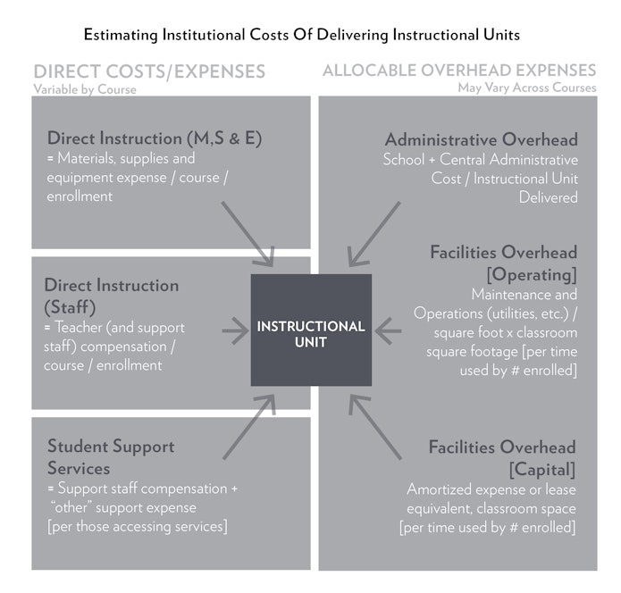
The right-hand side of Figure 2 addresses institutional expenses which may be “allocated” to instructional units based on an allocation factor. That is, we must determine an appropriate method for assigning expenses associated with administrative overhead, and plant operations to the delivery of courses and credits. We also must find a way to measure the extent to which students access student and academic support services and determine the expenses associated with those services.
Figure 3 presents an alternative perspective on the same task, as viewed from the perspective of plausible data sources. At the bottom of the first panel, we have the direct expenses associated with credits taken by students toward degree completion. These estimates are arrived at through evaluations of student course-taking behavior (from student transcripts, combined with scheduling and enrollment data systems) and personnel data (linking instructors, their qualifications and compensation to courses), which are represented in the second panel of the figure. Overhead expenses can be obtained from detailed institutional expenditure reports drawn from financial information systems and must then be formulaically allocated to courses. Less precise overhead expenses might be drawn from larger sets of institutions using financial data from the Integrated Postsecondary Education Data System (IPEDS).
Figure 3.
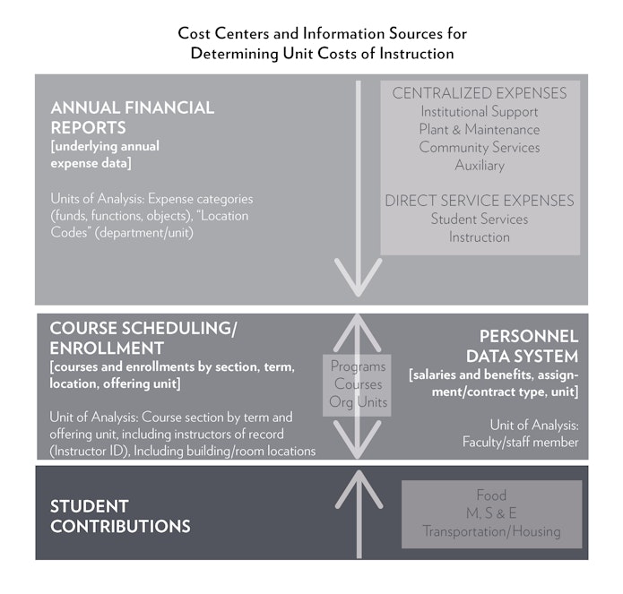
Importantly, if the goal of these analyses is to provide policy guidance regarding the costs of persistence and completion, we must also be able to estimate additional costs of attendance currently covered by students, including food (while on site), textbooks and other course materials, and transportation and housing, where applicable.
Expenditure analyses of the type described thus far could be readily carried out on one or a handful of selected community colleges. Romano and colleagues applied similar methods to a New York community college.63 The major limitation of these analyses, however, is that they merely describe their observations in a single or handful of institutions, given existing outcomes (sufficient or not) of existing populations (diverse or not) in existing contexts and at existing degrees of inefficiency.
From Pathway-Dependent Expenditure Summaries to Cost Estimates
What we have described thus far in this section is an analysis of the institutional “expenses” (not costs) associated with degree completion for one student or a group of students. That is, how much direct expense is attributed, and indirect expense allocated, to the credits consumed by students toward completing certain degree requirements? Taking the step toward cost analysis requires that we more thoroughly parse the relationship between the inputs used to provide the credits and associated spending, and the outcomes attained.
We will now review concepts laid out previously in this paper. Institutions might expend somewhat more than might be minimally necessary to achieve any given level of outcomes:
Cost = Expenditure – Inefficiency
But that doesn’t mean that existing institutional practices and expenditure data aren’t useful for distilling “costs.” In fact, they may be the only basis—the starting point—from which we can begin to understand costs. To accomplish this task, we must evaluate variations in institutional expenditures as they relate to variations in student outcomes, with consideration for the “risk” and “cost” factors addressed previously and while acknowledging that variations in inefficiency exist. That is, what do existing institutions spend to achieve selected, measured outcomes, taking into account environmental prices and other cost factors, and given who they serve? Or, expressed as a function:
Expenditure = f(Outcomes, Risk Factors, Input Prices, Scale, Type, Inefficiency)
We can leave it at that, assuming that the remaining spending variations not associated with outcome variations or cost and risk factors constitute inefficiency;64 or we can explore potential sources of inefficient expenditure, then statistically control for those factors when determining “costs.”65
Identifying the underlying absolute minimum cost at which any given set of outcomes can be produced is an unattainable goal. But that should not stop us from exploring the variations in expenditures across existing institutions and programs that share similar goals.
Much can be learned from variation in existing institutional production of student outcomes, with consideration for alternative student pathways toward those outcomes. As such, we must find ways to:
- conduct student pathway analyses simultaneously across multiple institutions, including similar programs across multiple institutions and contexts;
- combine these analyses with models of institutional expenditures, including those directly attributable to instructional programs as well as overhead expenses allocable to those programs; and
- identify outcome measures that better capture differences in the quality of outcomes rather than merely the quantity.
The first of these issues can most likely be addressed by applying cost analysis to large state systems, including multiple two-year public institutions offering the same types of programs, certifications and degrees, as well as common employee compensation data systems, common course coding systems and programmatic requirements, common chart of accounts for expenditures, and common measures of student outcomes. Where these conditions are met, one could determine the program within institution expenses associated with achieving common outcome goals, and further explore how those expenses vary from one institution to the next, and across different types of entering students. That is, one could discern whether the presumed risk and cost factors (addressed previously in this report) are associated with different expenses toward achieving common outcomes, and one could then attempt to distill differences in efficiency toward achieving common outcomes, given those risk and cost factors.
Where specific programs of study (within institutions) are the unit of analysis, one can more precisely match the outcome measures to programmatic goals: comparing degree completions across similar fields (with appropriate consideration for nuances),66 certificate completions across fields,67 and programs with similarly high rates of transfer.68 Further, where end-of-course exams and/or professional licensure exams exist, apples-to-apples comparisons of costs in relation to those measures may be made.
A second-best alternative involves applying more traditional cost models to institutions as the unit of analysis, as is usually the case in elementary and secondary education cost modeling. As Bahr has shown, community colleges may be classified by the types of programs and courses of study their students pursue, in part driven by the economic context in which they operate.69 Modeling institutional expenditures and outcomes, given risk and cost factors, for institutions of similar type (while applying relevant outcome metrics), may also provide useful insights, though with less precision than comparing specific programs across institutions would offer.
Conclusions & Policy Implications
In elementary and secondary education policy, the purpose of estimating costs is to directly inform policy—specifically, to inform the design of state aid formulas so that they provide for equal educational opportunity and educational adequacy. The policy goal to provide equal educational opportunity through state, intermediate (county), and local financing should be similar for community college education. Thus, the purpose of cost analysis in the post-secondary context is similar, but from a starting point where few, if any, systemwide cost analyses of community colleges have yet been conducted, and where cost and risk factors have yet to be fully vetted for their potential inclusion in targeted aid formulas. In translating the work of cost analysis from the elementary and secondary setting to post-secondary settings, we suggest the following guiding principles:
- Outcome goals must be sensitive to institutional goals and derivative of student choices and economic context.
- Policies must address all costs associated with successful persistence and completion of quality degree and certificate programs (including transportation, food, materials, supplies, etc.).
- Policies must provide sufficient resources to mitigate student risk factors, to equalize the likelihood of success regardless of student background factors.
- Policies must be sufficiently sensitive to regional variations in labor costs, costs associated with dis-economies of scale, and population sparsity.
We acknowledge that we cannot possibly prescribe the resources required for the perfectly efficient post-secondary institution, but that this unattainable objective should not interfere with our pursuit of reasonable estimates based on existing realities. Further, we suspect that producing cost analyses based on the collective professional judgment of scholars, practitioners, and the available research evidence in order to propose the hypothetically ideal community college, while certainly interesting, would be an overwhelming task given the limited body of evidence upon which to draw.
Thorough, well-constructed hybrid cost analyses may provide useful guidance for both state policymakers operating at the higher level at which policy decisions are made, and for institutional leaders closer to where services are actually delivered who are seeking guidance regarding effective resource allocation strategies. In the best case, top-down cost modeling driven by student pathway analysis that uses programs as the unit of analysis, coupled with detailed data on institutional overhead and related service costs, can provide us with (a) accurate and comprehensive estimates of the costs of achieving desired persistence and completion rates by program, and (b) estimates of which programs and institutions seem to be achieving better outcomes more efficiently or effectively. Importantly, this approach provides the opportunity for follow-up (and deep-dive) analyses of how those institutions allocate resources within their programs and distribute student services and institutional supports across programs.
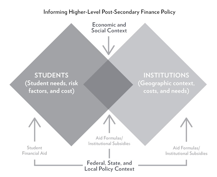
Figure 4 addresses the higher-level policy question of how program-specific cost estimates may inform public policy. Specifically, information on how costs vary across institutions by context and students served, coupled with information on local capacity to raise revenues, can inform the development of state aid formulas for community colleges. These aid formulas may include regional cost adjustment factors, adjustment for costs associated with the delivery of necessary small-scale programs and services (e.g., those in remote rural settings), and weights applied to institutional aid based on student populations served and additional support services necessary for their success. Because community college financing, unlike elementary and secondary financing, also involves direct student support via student financial aid, cost findings may also provide guidance on differentiating student aid by program, institution, and by individual needs and risk factors.
Figure 4.
At these early stages, it seems unlikely that convened panels of practitioners or policymakers could engage in developing bottom-up specifications of the resources required to provide adequate, equitable community college education across the array of existing program and institutional types. More speculative yet, it would be extremely difficult for expert practitioners working in isolation to develop improved institutional structures under which adequate community college programs might be provided in an equitable manner. However, we firmly believe that there are many lessons to be learned from examining existing variations across institutions and programs, including from detailed information on how those institutions deploy and compensate full-time and part-time faculty, how student support services are delivered, how faculty supports are organized, and how department and institutional administrative structures are organized. Specific programs and institutions identified as especially productive and efficient with certain students and in certain contexts should therefore be used to generate detailed resource and expenditure profiles which may provide useful guidance for local, institutional leaders, as well as for state policymakers.
Much can and should be learned from the ways in which existing institutions organize their resources, and the manner in which students access those resources, toward achieving their respective institutional and individual goals and broader societal and economic contributions. Some institutions are more effective than others at achieving these goals and some students choose more efficient paths than others. At the intersection are institutional structures that enable and encourage individuals to pursue their most efficient pathways to their desired outcomes.
Cost analyses must be ongoing and cyclical to support policy refinement. As institutions adapt and change in the presence of shared information on costs, those adaptations may influence the next cycle of cost analyses—perhaps revealed as improved efficiency. With institutions like community colleges so highly responsive to local economic contexts, changes to those contexts may also influence cost estimates over time. As the student populations entering community colleges in general, and specific degree and certificate programs in particular, change, so too do the costs of meeting their needs. Finally, as the role community colleges play in society at large changes and as the outcome goals of community colleges evolve, so too do the costs of achieving those goals. The end goal must not merely be to make community college more equally accessible but to provide for a system which ensures that all that enter have equal opportunity to persist, complete and achieve their desired outcomes.
This report is the first in a series by the Century Foundation’s Working Group on Community College Financial Resources. This report was published with the generous support of the WT Grant Foundation.
Appendix A – Evaluating Reliability and Validity
Far too little attention has been paid to methods for improving reliability and validity in education cost analysis. In this context, we evaluate validity and reliability as follows:
Validity: Does the cost estimate really reflect what goes into producing the desired level, depth, and breadth of educational outcomes?
Reliability: Are the costs measured consistently over time, across methods or when applied by different individuals or teams?
These two must go hand in hand, or at least reliability should be contingent on validity, because a finding can be reliably wrong (i.e. measuring the wrong thing, but consistently). Baker (2006) and Duncombe (2006, 2011) proposed steps to strengthen the reliability and validity of education cost studies, especially when applied in the context of estimating the costs of achieving specific educational outcomes, or educational “adequacy.”70
Validity takes many forms, the simplest of which is “face validity.” That is, on its face, does the estimate measure what it purports to measure? Where the goal is to measure the costs of achieving specific state standards, arguably, the Evidence-Based approach of aggregating research findings on strategies implemented in entirely different settings, and evaluated by entirely different outcomes, fails to achieve face validity. This is not to suggest, however, that context-specific focus group recommendations formulated through a Professional Judgement approach that do not take into account any research evidence are superior. Some hybrid of the two, with additional validation, is warranted.
Predictive validity asks whether the cost estimates are actually predictive of the spending levels required for achieving desired outcomes and should be included in any cost analysis. Baker (2006), Chambers, Levin & Parrish (2006), and Levin and Chambers (2009) explain that one weak predictive validity check on educational adequacy cost studies is the evaluation of whether those schools and districts identified as having funding shortfalls—that is, those that have less than they need for achieving “adequate” educational outcomes—do in fact achieve less than adequate outcomes, while those having more than adequate resources exceed adequate outcomes, and further, whether the magnitude of the resource deficits or surpluses correlates with the magnitude of the outcome deficits or surpluses.71 Such checks and balances are especially warranted in focus group-driven RCM analyses, where the association with outcomes is more speculative, or hypothetical. In cases where the relationship between input gaps and outcome gaps is very weak, findings are particularly vulnerable to skeptics, and legitimately so.72
For focus group-driven RCM, the hypotheses of resources needed for achieving desired outcomes might be validated by comparison with the resources of actual schools and districts, as estimated via cost function modeling, that actually achieve the desired outcome levels with profiles of spending and resource use that mirror that of the RCM-prescribed model.
Finally, specific to ECF modeling, alternative models should be tested for their ability to accurately predict the spending behavior of districts excluded from the model. With complex statistical models having many variables and moving parts, it is important to identify a model that is sufficiently generalizable. In this case, “sufficiently generalizable” means that the model characterizes well the patterns of relationship among conditions, students, resources, and outcomes, such that the model can be used to predict the spending levels needed to achieve desired outcomes under different conditions.73
Alternatives for reliability checks are also relatively straightforward. Exclusively within a focus group-driven RCM format, one might convene independent panels that are provided similar tasks (identifying resources needed to meet a particular set of outcomes X, Y, and Z under specific conditions A, B, and C) and then compare findings across panels. That is, conduct a within-method reliability check. Alternatively, one might evaluate the correlation between findings across the RCM and ECF approaches. But again, reliability is of little concern in the absence of reasonable validity checking.
Notes
- Adam Tamburin, “House approves Haslam’s tuition-free college plan,” the Tennessean, April 13, 2017, http://www.tennessean.com/story/news/education/2017/04/13/house-approves-haslams-tuition-free-college-plan/100417716/
- Scott Jaskin, “New York Adopts Free Tuition,” Inside Higher Ed, April 10, 2017, https://www.insidehighered.com/news/2017/04/10/new-york-state-reaches-deal-provide-free-tuition-suny-and-cuny-students
- Michael Leachman and Chris Mai, “Most states still funding schools less than before the recession,” Center on Budget and Policy Priorities, October 14, 2014, https://www.cbpp.org/research/most-states-still-funding-schools-less-than-before-the-recession
- Bruce Baker, “School Funding Fairness in New York State: An Update for 2013-14,” Alliance for Quality Education, January 24, 2014, http://www.aqeny.org/wp-content/uploads/2012/03/School-Funding-Fairness-in-New-York-State-An-Update-for-2013-14.pdf
- Bruce Baker et al, “Is School Funding Fair? A National Report Card,” Education Law Center, January, 2017, http://www.edlawcenter.org/assets/files/pdfs/publications/National_Report_Card_2017.pdf
- Ibid.
- Robert Berne and Leanna Stiefel, “The Equity of School Finance Systems over Time: the Value Judgments Inherent in Evaluation,” Educational Administration Quarterly 15, no. 2, 1979, 14-34.
- Robert Berne and Leanna Stiefel, The Measurement of Equity in School Finance: Conceptual, Methodological and Empirical Dimensions (Baltimore, MA: Johns Hopkins University Press 1984); Robert Berne and Leanna Stiefel, “Concepts of School Finance Equity: 1970 to the Present,” Equity and Adequacy in Education Finance: Issues and Perspectives (Washington, D.C.: National Academy Press, 1984), 7-33.
- Regarding children with disabilities, see: Endrew F.. v. Douglas County School District RE-1, 580 U.S. (2017). Regarding children with limited English language proficiency, see: Issa v. School District of Lancaster, U.S. 3rd Circuit 16-3528 (2017).
- Bruce Baker and Preston Green, “Conceptions, measurement and application of educational adequacy standards,” AERA handbook on education policy (New York: Routledge, 2009), 311-337; Bruce Baker and Preston Green, “Conceptions of equity and adequacy in school finance,” Handbook of Research in Education Finance and Policy, eds Helen Ladd and Margaret Goertz, (New York: Routledge, 2008), 203-221.
- William Clune, “The Shift from Equity to Adequacy in School Finance,” Educational Policy 8, no. 4 (1994): 376-394.
- William Koski and Rob Reich, “When Adequate Isn’t: The Retreat from Equity in Educational Law and Policy and Why It Matters,” Emory Law Journal 56, no.3 (2007): 545.
- For example, the Kansas Constitution requires that the legislature “shall make suitable provision for finance of the educational interests of the state.” Those educational interests are articulated in standards adopted by the state board of education (which holds independent constitutional authority for the “general supervision of public schools”). Kansas courts have repeatedly held that the legislature’s obligation is to provide financing which grants all children equal opportunity to achieve those standards. Gannon v. State, 368 P.3d 1024, 303 Kan. 682 (2016); Gannon v. State, No. 113, 267 Kan. (June 28, 2016); Montoy v. State, 279 Kan. 817, 112 P.3d 923 (2005); USD NO. 229 v. State, 256 Kan. 232, 885 P.2d 1170 (1994).
- Avidan Cover, “Is Adequacy a More Political Question Than Equality: The Effect of Standards-Based Education on Judicial Standards for Education Finance,” Cornell Journal of Law and Public Policy 11, no. 2 (2002): 403.
- Michael Rebell, “Safeguarding the right to a sound basic education in times of fiscal constraint,” Albany Law Review 75 (2011): 1855.
- Bruce Baker and Preston Green, “Conceptions of Equity,” 203-221; Bruce Baker and Preston Green, “Conceptions, Measurement and Application,” 311-337.
- Rose v. Council for Better Educ., Inc., 790 S.W.2d 186, 60 Ky. 1289 (1989).
- Andrew Porter and Morgan Polikoff, “Measuring Academic Readiness for College,” Educational Policy 26, no. 3 (2012):, 394-417; Peter Conforti, “What Is College and Career Readiness? A Summary of State Definitions,” Pearson Bulletin 22 (2013): 1-4.
- William Duncombe and John Yinger, “Performance Standards and Educational Cost Indexes: You Can’t Have One Without the Other,” Equity and Adequacy in Education Finance: Issues and Perspectives 260 (1999): 261.
- An emerging body of literature on value-added contributions of post-secondary institutions exists: Ou Liu, “Value-added assessment in higher education: A comparison of two methods,” Higher Education 61, no. 4 (2010): 445-461; Jesse Cunha and Trey Miller, “Measuring Value-Added in Higher Education: Possibilities and Limitations in the Use of Administrative Data,” Economics of Education Review 42 (2014): 64-77; Ou Liu, “Measuring value‐added in higher education: conditions and caveats–results from using the Measure of Academic Proficiency and Progress (MAPP™),” Assessment & Evaluation in Higher Education, 36, no. 1 (2011): 81-94; Richard Shavelson et al, “On the practices and challenges of measuring higher education value added: the case of Colombia,” Assessment & Evaluation in Higher Education 41, no. 5 (2016): 695-720.
- Bruce Baker and Preston Green, “The Politics of School Finance in the New Normal Era,” Handbook of Education Politics and Policy (New York: Routledge, 2014), 166.
- Robert Rothman, “A Common Core of Readiness,” Educational Leadership 69, no. 7 (2012): 10-15.
- Bruce Baker et al, “The Effect of Labor Market Information on Community College Students’ Major Choice,” (presentation, ASSA Annual Meeting: Major Choices: Students’ Beliefs About Labor Market Outcomes, American Economic Association, Ann Arbor, MI, April, 2017).
- Campaign for Fiscal Equity, Inc. v. State, 2006 N.Y. Slip Op 8630 (2006).
- “Community Colleges Outcomes Report: the Role of Community Colleges in Postsecondary Success,” National Student Clearinghouse Research Center, 2017, https://studentclearinghouse.info/onestop/wp-content/uploads/Comm-Colleges-Outcomes-Report.pdf
- Doug Shapiro et al, “Completing College: A National View of Student Attainment Rates–Fall 2008 Cohort (Signature Report No. 8),” National Student Clearinghouse, 2014, https://nscresearchcenter.org/wp-content/uploads/SignatureReport8.pdf ; See also: Susan Dynarski, Steven Hemelt, and Joshua Hyman, “The missing manual: Using National Student Clearinghouse data to track postsecondary outcomes,” National Bureau of Economic Research, October, 2013, http://www-personal.umich.edu/~jmhyman/dynarski_hemelt_hyman_missing_manual.pdf
- Christopher Jepsen, Kenneth Troske, and Paul Coomes, “The Labor-Market Returns to Community College Degrees, Diplomas, and Certificates,” Journal of Labor Economics 32, no. 1 (2014): 95-121; Mina Dadgar and Madeline Weiss, “Labor Market Returns to Sub-Baccalaureate Credentials: How Much Does a Community College Degree or Certificate Pay?” Educational Evaluation and Policy Analysis 37, no. 4 (2015): 399-418.
- Peter Bahr, “Labor Market Returns to Community College Awards: Evidence from Michigan. A CAPSEE Working Paper,” Center for Analysis of Postsecondary Education and Employment, March, 2015, https://capseecenter.org/wp-content/uploads/2015/03/labor-market-returns-michigan.pdf; Christopher Jepsen, Kenneth Troske, and Paul Coomes, “The labor-market returns,” 95-121.
- Peter Bahr, “The labor market return in earnings to community college credits and credentials in California” (working paper, Center for the Study of Higher and Postsecondary Education, University of Michigan, 2014).
- Ibid.
- Peter Bahr, “Classifying community colleges based on students’ patterns of use,” Research in Higher Education 54, no. 4 (2013): 433-460.
- Ibid; Bruce Ingraham, “Frequent Patterns in California Community College Student Course Sequences” (dissertation, Kalmanovitz School of Education, Saint Mary’s College of California, 2016).
- William Duncombe and John Yinger, “Measurement of Cost Differentials,” Handbook of Research in Education Finance and Policy, eds Helen Ladd and Margaret Goertz, (New York: Routledge, 2008), 238-256.
- Lori Taylor and William Fowler, Jr., “A Comparable Wage Approach to Geographic Cost Adjustment. Research and Development Report,” National Center for Education Statistics, May, 2006, https://nces.ed.gov/pubs2006/2006321.pdf
- Matthew Andrews, William Duncombe, and John Yinger, “Revisiting economies of size in American education: are we any closer to a consensus?” Economics of Education Review 21, no. 3 (2002): 245-262.
- Jay Chambers, “The Hedonic Wage Technique as a Tool for Estimating the Costs of School Personnel: A Theoretical Exposition with Implications for Empirical Analysis,” Journal of Education Finance 6, no. 3 (1981): 330-354.
- William Duncombe and Dan Goldhaber, “Adjusting for Geographic Differences in the Cost of Educational Provision in Maryland” (report prepared for the State of Maryland, December 31, 2003).
- Lori Taylor and William Fowler, Jr., “A Comparable Wage Approach.”
- Jay Chambers, “The Hedonic Wage Technique,” 330-354.
- Christopher Morphew and Bruce Baker, “On the Utility of National Datasets and Resource Cost Models for Estimating Faculty Instructional Costs in Higher Education,” Journal of Education Finance 33, no. 1 (2007): 20-48.; Susan Twombly and Barbara Townsend, “Community College Faculty What We Know and Need to Know,” Community College Review 36, no. 1 (2008): 5-24.
- Matthew Andrews, William Duncombe, and John Yinger, “Revisiting economies of size,” 245-262.
- Jennifer Imazeki, “Grade-Dependent Costs of Education: Evidence from Illinois” (draft paper, San Diego State University, 2001).
- Timothy Gronberg, Dennis Jansen, and Lori Taylor, “The Impact of Facilities on the Cost of Education,” National Tax Journal 64, no. 1 (2011): 193.
- Paul Brinkman and Larry Leslie, “Economies of Scale in Higher Education: Sixty Years of Research,” The Review of Higher Education 10, no. 1 (1986): 1.
- Christopher Morphew and Bruce Baker, “On the Utility of National Datasets,” 20-48.
- William Duncombe and John Yinger, “How much more does a disadvantaged student cost?” Economics of Education Review 24, no. 5 (2005): 513-532.
- Katherine Michelmore and Susan Dynarski, “The Gap within the Gap: Using Longitudinal Data to Understand Income Differences in Student Achievement,” National Bureau of Economic Research, July, 2016.
- Bruce Baker, “Exploring the Sensitivity of Education Costs to Racial Composition of Schools and Race-Neutral Alternative Measures: A cost Function Application to Missouri,” Peabody Journal of Education 86, no. 1 (2011): 58-83.
- Gloria Crisp and Chryssa Delgado, “The Impact of Developmental Education on Community College Persistence and Vertical Transfer,” Community College Review 42, no. 2 (2013): 99-117; Deryl Hatch and Crystal Garcia, “Academic Advising and the Persistence Intentions of Community College Students in their First Weeks in College,” The Review of Higher Education 40, no. 3 (2017): 353-390; Carlton Fong, Taylor Acee, and Claire Weinstein, “A Person-Centered Investigation of Achievement Motivation Goals and Correlates of Community College Student Achievement and Persistence,” Journal of College Student Retention: Research, Theory & Practice, October, 2016, https://doi.org/10.1177/1521025116673374
- Oscar Jimenez-Castellanos, Amelia Topper, “The cost of providing an adequate education to English language learners: A review of the literature,” Review of Educational Research 82, no. 2 (2012): 179-232.
- Jay Chambers and Jean Wolman, “What Can We Learn from State Data Systems about the Cost of Special Education? A Case Study of Ohio,” Center for Special Education Finance, John C. Flanagan Center at the American Institutes for Research, September, 1998.
- Forthcoming work by Toutkoushian suggests that while first-generation students may struggle to complete four-year undergraduate programs, they may perform better (including better than their peers) in some community college settings.
- “Study by Stella Flores Finds More Than Half of the Racial College Completion Gap Explained by Pre-College Factors,” At a Glance: News from the Steinhardt School of Culture, Education, and Human Development, April 6, 2017, http://steinhardt.nyu.edu/site/ataglance/2017/04/study-by-stella-flores-finds-more-than-half-of-the-racial-college-completion-gap-explained-by-pre-college-factors.html; Stella Flores, Toby Park, and Dominique Baker, “The Racial College Completion Gap: Evidence from Texas,” The Journal of Higher Education 88, no. 6 (2017): 1-28.
- Ibid.
- For a review of cost function analyses, see: William Duncombe and John Yinger, “Are Education Cost Functions Ready for Prime Time? An Examination of Their Validity and Reliability,” Peabody Journal of Education 86, no. 1 (2011): 28-57; Timothy Gronberg, Dennis Jansen, and Lori Taylor, “The Adequacy of Educational Cost Functions: Lessons from Texas,” Peabody Journal of Education 86, no. 1 (2011): 3-27.
- Lars-Erik Borge, Torberg Falch, and Per Tovmo, “Public sector efficiency: the roles of political and budgetary institutions, fiscal capacity, and democratic participation,” Public Choice 136, no. 3-4 (2008): 475-495; Shawna Grosskopf et al, “On the Determinants of School District Efficiency: Competition and Monitoring. Journal of Urban Economics 49, no. 3 (2001): 453-478.
- John Sonstelie, “Aligning School Finance With Academic Standards: A Weighted-Student Formula Based on a Survey of Practitioners” (occasional paper, Public Policy Institute of California, March, 2007).
- Overly confident efforts to suggest otherwise have been met with sharp ridicule. See: Eric Hanushek, “The Confidence Men: Selling Adequacy, Making Millions,” Education Next 7, no. 3 (2007).
- Jay Chambers, “The Patterns of Services Provided to Students with Disabilities,” American Institutes for Research in the Behavioral Sciences, 1998, http://files.eric.ed.gov/fulltext/ED425568.pdf; Jay Chambers and Jean Wolman, “What Can We Learn from State Data Systems;” Jay Chambers, “Measuring Resources in Education: From Accounting to the Resource Cost Model Approach” (working paper, US Department of Education, Office of Educational Research and Improvement, National Center for Education Statistics, June, 1999).
- Jay Chambers, “The Patterns of Services.”
- Christopher Morphew and Bruce Baker, “On the Utility of National Datasets,” 20-48.
- Susan Dynarski, Steven Hemelt, and Joshua Hyman, “The Missing Manual.”
- Richard Romano, Regina Losinger, and Tim Millard, “Measuring the Cost of a College Degree: A Case Study of a SUNY Community College,” Community College Review 39, no. 3 (2011): 211-234.
- Tommaso Agasisti and Clive Belfield, “Efficiency in the Community College Sector: Stochastic Frontier Analysis,” Tertiary Education and Management 23, no. 3 (2017): 1-23. See also: Clive Belfield, “Measuring Efficiency in the Community College Sector. CCRC Working Paper No. 43,” Community College Research Center, Columbia University, April, 2012, http://files.eric.ed.gov/fulltext/ED531229.pdf
- Recall that variations in inefficiency across local government agencies are commonly presumed to be a function of variations in (a) public monitoring, (b) fiscal capacity, and (c) competition density.
Inefficiency = f(Public Monitoring, Competition, Fiscal Capacity) - Elisa Rassen et al, “Nuances of completion: Improving student outcomes by unpacking the numbers,” Community College Research Center, Columbia University, April 2013, https://ccrc.tc.columbia.edu/media/k2/attachments/nuances-completion-student-outcomes-cbd.pdf; Thomas Bailey et al, “The Effects of Institutional Factors on the Success of Community College Students,” Community College Research Center, Columbia University, February, 2005.
- Di Xu and Madeline Trimble, “What About Certificates? Evidence on the Labor Market Returns to Non-degree Community College Awards in Two States,” Educational Evaluation and Policy Analysis 38, no. 2 (2016): 272-292.
- Peter Bahr et al, “A Review and Critique of the Literature on Community College Students’ Transition Processes and Outcomes in Four-Year Institutions,” Higher Education: Handbook of Theory and Research (Netherlands: Springer, 2013), 459-511; Scott Carrell and Michael Kurlaender, “Estimating the Productivity of Community Colleges in Paving the Road to Four-Year College Success,” Productivity in Higher Education (Chicago: University of Chicago Press, 2017); Davis Jenkins and John Fink, “Tracking Transfer: New Measures of Institutional and State Effectiveness in Helping Community College Students Attain Bachelor’s Degrees,” Community College Research Center, Teachers College, Columbia University, January, 2016.
- Peter Bahr, “Classifying Community Colleges.” The categories of “Community Education Intensive,” “Transfer Intensive,” “Workforce Development Intensive,” “High-Risk Intensive,” and “Mixed Use” come from this paper.
- Bruce Baker, “Evaluating the Reliability, Validity, and Usefulness of Education Cost Studies,” Journal of Education Finance 32, no. 2 (2006): 170-201.; William Duncombe, “Responding to the Charge of Alchemy: Strategies for Evaluating the Reliability and Validity of Costing-Out Research,” Journal of Education Finance 32, no. 3 (2006): 137-169.; William Duncombe and John Yinger, “Are Education Cost Functions Ready,” 28-57.
- Bruce Baker, “Evaluating the Reliability,” 170-201.; Jay Chambers, Jesse Levin, and Thomas Parrish, (2006), “Examining the Relationship between Educational Outcomes and Gaps in Funding: An Extension of the New York Adequacy Study,” Peabody Journal of Education, 81, no. 2 (2006): 1–32.;Jay Chambers and Jesse Levin, “Determining the Cost of Providing an Adequate Education for All Students,” National Education Association, 2009.
- Eric Hanushek, “The Alchemy of ‘Costing Out’ an Adequate Education,” presented at Adequacy Lawsuits: Their Growing Impact on American Education, Kennedy School of Government, Harvard University, October 13-14, 2005.; Eric Hanushek, “Science Violated: Spending Projections and the ‘Costing Out’ of an Adequate Education,” Courting Failure: How School Finance Lawsuits Exploit Judges’ Good Intentions and Harm Our Children (Palo Alto, CA: Education Next Books, 2006), 257-312.; Robert Costrell, Eric Hanushek, and Susanna Loeb, “What do cost functions tell us about the cost of an adequate education?” Peabody Journal of Education 83, no. 2, (2008): 198-223.
- One can test the generalizability of alternative cost models by splitting the sample of schools or districts in a state into two groups, fitting a model to one group, and then using it to predict the spending of the other. For an application of this type of validity testing, see: Bruce Baker, “Exploring the Sensitivity of Education Costs.” One can either split the sample down the middle, or into a smaller group for prediction checking, using the larger group for model-fitting. This predictive validity check is commonly referred to as the split-cross validation method. Alternatively, one can hold back subsequent years of data for prediction testing and use prior years to fit the model. See William Duncombe, “Responding to the Charge of Alchemy.”