
There has been considerable interest in financial transactions taxes (FTTs) in the United States and other wealthy countries in the years since the financial crisis. An FTT can be a way to both raise a large amount of revenue and also rein in the financial sector. This report examines the evidence on the potential for raising revenue through an FTT, its impact on the economy, and also the possibility of using the revenue to defray in particular the cost of higher education. The report argues:
- A financial transactions tax could likely raise over $105 billion annually (0.6 percent of GDP) based on 2015 trading volume. This estimate is roughly in the middle of recent estimates that ranged from as high as $580 billion to as low as $30 billion.
- The full amount of this tax would be borne by the financial industry, and not individual holders of stock or pension funds and other institutional investors. Evidence suggests that trading volume is elastic with respect to price, meaning that any drop in trading volume resulting from the tax would reduce costs for end users by a larger amount than the tax would increase them.
- It is reasonable to believe that the industry would be no less effective in serving its productive use (allocating capital) after the tax is in place. This means that one of the primary effects of the tax would be to reduce waste in the financial sector, reducing costs while having little or no effect on its principal purpose: to allocate capital effectively.
- The revenue raised through an FTT would easily be large enough to cover the cost of free college tuition (among other social programs), although if nothing were done to stem the growth rate of college costs, it would eventually prove inadequate.
The report also notes that the financial sector is the main source of income for many of the highest earners in the economy. This means that downsizing the industry through an FTT could play an important role in reducing income inequality.
Introduction
Financial transactions taxes (FTTs)—levies on a nation’s monetary transactions, such as securities trading—can be an effective way to raise large amounts of revenue. And they can do so without harming the workings of financial markets. Since the 2008 financial crisis, in the United States and abroad, there has been growing interest in FTTs, both as a source of revenue and as a tool for reining in the financial sector.
Ten countries in the eurozone have been trying to work through the details of a multi-tiered tax that would apply differing tax rates to various financial instruments. In the meantime, both France and Italy have jumped ahead, imposing a financial transactions tax of 0.2 percent and 0.1 percent, respectively, on equity trades.1
In the United States in 2010, then-Senator Tom Harkin and Representative Peter DeFazio put forward a bill that would tax most financial transactions at a 0.03 percent rate. More recently, Senator Bernie Sanders made a financial transactions tax one of the centerpieces of his presidential campaign, proposing a multi-tiered tax as a mechanism to finance his plan to make college education free.
There are a variety of reasons for advocating for FTTs. The most obvious one is to raise revenue. Clearly, FTTs can raise a substantial amount of revenue, although there is considerable dispute around the plausible range. At the high end, a recent study by Robert Pollin, James Heintz, and Thomas Herndon at the Political Economy Research Institute of the University of Massachusetts (referred to simply as PHH from here on) calculated that a financial trade transaction tax along the lines proposed by Senator Sanders could raise more than $340 billion annually, or just under 2.0 percent of GDP. 2 A study by Austrian economist Stephan Schulmeister calculated that a tax could raise 3.2 percent of GDP, which would be almost $580 billion in the 2016 U.S. economy.3
A study by the Leonard Burman and his colleagues at the Tax Policy Center of the Brookings Institution and the Urban Institute (referred to simply as Burman from here on) came in with a much lower figure, concluding that a tax would likely raise less than $40 billion annually.4 The Joint Tax Committee projected that the more modest tax proposed by Harkin and DeFazio could raise $30 billion a year.
It is also worth noting the other rationales that have been put forward for FTTs. In addition to the revenue potential, many have argued for FTTs as a way to reduce volatility in financial markets. The argument is that by discouraging short-term trading, the volatility in markets would be reduced. Yet another argument is that by reducing the volume of trading, FTTs would reduce the resources wasted in the financial sector. If the reduction in trading volume does not impede the ability of financial markets to serve the real economy, then an FTT would effectively make the sector more efficient. Finally, FTTs are sometimes suggested as a way to reduce short-termism. The argument is that by lengthening the time horizon of actors in financial markets, FTTs would also lengthen the time horizon of corporate management, leading to better management decisions.
This report will briefly discuss these other rationales, but focuses first on the revenue-generating potential of the tax. The first section provides a detailed assessment of the basis for the differences in revenue projections across studies and produces its own set of projections. The second section discusses the way in which FTTs reduce waste in the financial sector. This has been a topic of much confusion and deserves a careful treatment. The third section discusses the economic impact of an FTT and whether it will affect capital investment and other related economic issues. The fourth section discusses the implications of Senator Sanders’ proposal used as a case study, to cover the costs of making public colleges tuition free.
Section I: The Revenue Potential of Financial Transactions Taxes
This section provides a short summary of existing research and evidence on the revenue potential of FTTs. Based on this analysis, this report models a tax on stock trades of 0.2 percent, a tax on bond trades of 0.1 percent, and a tax on derivative trades of 0.002 percent of their nominal value. In total, this report estimates such a tax will raise $120 billion in the first year, as noted above.
Financial transactions taxes are hardly new to the world, or even the United States. Most countries with stock markets have imposed FTTs for most of their existence. The United Kingdom began imposing a stamp tax on stock trades in 1694. Traders paid to get the stamp from the government, which was necessary to have a legal transaction. This stamp tax continues to the present, with a rate of 0.5 percent per trade. The tax raises an amount of revenue that averages more than 0.2 percent of the U.K.’s GDP (the equivalent of $36 billion annually in the United States in 2016). Until the early 1990s, Japan imposed a multi-tiered tax that applied across most financial instruments. At the peak of Japan’s stock bubble in 1990, the tax raised more than 1.0 percent of GDP.5
The United States also has experience with FTTs. Until 1966, it imposed a stamp tax of 0.04 percent on stock trades and 0.1 percent on newly issued shares of stock. Although this tax was removed, the Securities and Exchange Commission (SEC) continues to be funded by a tax of 0.0042 percent on stock trades.6 This tax raises roughly $500 million annually. Given this history, proposals to use FTTs to raise larger amounts of revenue should not seem radical.
Table 1 shows a subset of FTTs that are now in place around the world or have been in place in recent decades.7
| TABLE 1. REVENUES FROM FTTS, SELECTED G20 AND OTHER COUNTRIES (PERCENT OF GDP) | |||||||||||
| Country | 1990 | 1995 | 2000 | 2001 | 2002 | 2003 | 2004 | 2005 | 2006 | 2007 | 2008 |
| France | 0.051 | 0.010 | 0.028 | 0.019 | 0.015 | 0.014 | 0.012 | 0.012 | 0.013 | 0.014 | elim |
| Germany | 0.062 | 0.001 | elim | elim | elim | elim | elim | elim | elim | elim | elim |
| Hong Kong | na | na | na | na | na | na | na | na | na | na | 2.100 |
| India | na | na | na | na | na | na | 0.019 | 0.074 | 0.117 | 0.118 | 0.103 |
| Italy | 0.076 | 0.120 | elim | elim | elim | elim | elim | elim | elim | elim | elim |
| Japan | 0.175 | 0.105 | elim | elim | elim | elim | elim | elim | elim | elim | elim |
| South Korea | 0.102 | 0.179 | 0.615 | 0.372 | 0.450 | 0.319 | 0.216 | 0.411 | 0.434 | 0.577 | na |
| South Africa | na | na | na | 0.337 | 0.360 | 0.360 | 0.462 | 0.536 | 0.582 | 0.494 | 0.506 |
| Switzerland | 0.563 | 0.382 | 0.851 | 0.666 | 0.504 | 0.457 | 0.471 | 0.444 | 0.463 | 0.461 | na |
| Taiwan | na | na | na | 0.651 | 0.773 | 0.720 | 0.846 | 0.646 | 0.792 | 1.066 | 0.767 |
| UK | 0.120 | 0.170 | 0.450 | 0.270 | 0.230 | 0.220 | 0.220 | 0.270 | 0.280 | 0.290 | 0.220 |
| Source: Thornton Matheson, “Security transaction taxes: issues and evidence,” International Tax and Public Finance 19, no. 6 (2012): 884–912, Table 2. Note: na = not available; elim = eliminated. | |||||||||||
Table 1 is useful because it shows that FTTs have been effective in raising a substantial amount of revenue in a wide variety of countries. It also provides some insight into the potential revenue that can be raised from an FTT in the United States. The example of the U.K. is instructive. The tax only applies to stock trades, not to derivatives or bonds. Yet it consistently raised an amount of revenue that was well over 0.2 percent of GDP in the years from 2000 to 2008, with a peak of 0.45 percent at the height of the stock bubble in 2000.8 In the context of the U.S. economy in 2016, the peak of 0.45 percent of GDP would be equal to $81 billion.
The highest figures are the 1.07 percent of GDP shown for Taiwan in 2007 and the 2.1 percent of GDP shown for Hong Kong in 2008. The latter figure seems to be somewhat of an outlier, since revenue in Hong Kong from the tax fell to 1.3 percent of GDP the following year.9 Even excluding the Hong Kong figure for 2008, the table indicates that it has been possible to collect revenue in excess of 1.0 percent of GDP from an FTT. In addition to the high revenue collections shown for Hong Kong and Taiwan, the revenue collected from Switzerland in the years in the table since 2000 averaged well over 0.5 percent of GDP. This means that if a U.S. FTT is as effective as collecting revenue as the Swiss tax, then it would raise close to $90 billion in the 2016 economy. If the tax were as effective as the taxes in Taiwan and Hong Kong, then it could raise more than 1.0 percent of GDP, or $180 billion in the 2016 economy.10
There are four main factors in determining the potential revenue from an FTT:
- The current volume of trading;
- The current level of transactions costs;
- The elasticity of trading volume with respect to transactions costs; and
- The tax rate applied and the design of the tax.
These factors are discussed primarily in the context of the recent studies by Burman and by PHH. The assessment here is that the first study produces an estimate of potential revenue that is too low, because it understates the actual volume of transactions in financial markets. The latter study overstates potential revenue from an FTT, primarily because it overstates current transactions costs, which leads it to underestimate the extent to which trading volume would fall in response to an FTT.
There can be large differences in assumptions on trading volume and transactions costs because our data in these areas is not very good, since much of this information is not publicly available. As a result, it is necessary to rely to some extent on proprietary sources and inferences from other data. The fourth factor noted above—the optimal tax rates and the design of the tax—depends in large part on the prior three factors. In order to determine the optimal tax rate, it is essential to have some idea of the current level of transactions costs as well as the elasticity of trading volume with respect to costs.11 These issues are addressed in order below.
Current Trading Volume
Table 2 shows the underlying trading amounts assumed in the revenue calculations in PHH and in Burman, the most careful analyses of the revenue potential for an FTT in the United States.
| TABLE 2. TRADING COLUME UNDERLYING CALCULATIONS (BILLIONS OF DOLLARS) | ||
| Burman et. all | PHH | |
| Stocks | $33,794 | $48,000 |
| Bonds | $182,332 | $180,000 |
| Derivatives | $235,573 | $5,200,000 |
| Source and notes: Burman et al. (2016) and Pollin et al. (2016) (PHH). | ||
The data for PHH are for 2015, while the data for Burman are from 2014. This difference in years can explain some of the difference in the assumptions on current trading volume. As can be seen, the two studies use very similar assumptions for bond trading volume, with the difference quite plausibly attributable to the different years used. The PHH study assumes that trading in stock is nearly 50 percent higher than in Burman. Fortunately, there seems to be a simple explanation for most of this difference. PHH included trading volume from all the exchanges for which the Securities Industry and Financial Markets Association (SIFMA) provides data. By contrast, Burman appears to only have data on trading from the NYSE and NASDAQ.
Including trading volume from the other exchanges makes up most of the gap between the two assumptions on trading volume. SIFMA provides data on average daily trading volume by month.12 Multiplying the average daily volumes by 21 days (implying 252 trading days in a year) gives a figure of $44,956 billion in trading for 2015.
While determining the basis for the differences in assumptions on trading volume for stock is relatively easy, the problem with derivatives is far more difficult. Burman obtained data on trading by type of derivative by using the sources and methods described in a 2009 study by the Center for Economic and Policy Research.13 This led them to use an assumption of $235.6 trillion for the notional value of trades in the U.S. derivative market in 2014. By contrast, PHH derives a figure of $5,250 trillion for the notional value of derivative trades in the U.S. market in 2015, a number that is more than an order of magnitude larger.
Fortunately, PHH describes in detail the derivation of its assumption on trading volume. The study uses data on turnover and outstanding positions for exchange traded derivatives from the Bank for International Settlements (BIS) data on Exchange Trade Derivatives.14 It then gets data on outstanding positions on over-the-counter (OTC) derivatives from the BIS Global Derivative Statistics.15 While this source provides data on outstanding positions, it does not provide data on turnover. PHH assume that the turnover in the over-the-counter market is half as frequent as for exchange traded derivatives. The assumed turnover in the OTC market accounts for the bulk of the trading of derivatives in PHH.
There is actually data available from BIS on turnover in the OTC derivative market.16 These data show that OTC derivatives actually trade at between one-tenth and one-twentieth the frequency of exchange traded derivatives. This leads to a considerably smaller trading volume than assumed by PHH. Taking the value of exchange traded derivatives in the United States for 2015 and adding the value of OTC trading for 2013 gives $1.3 trillion.17
There is some room for uncertainty around this figure, but it seems clear that the assumed trading volume for derivatives in Burman is too low and the volume in PHH is too high. As noted earlier, there is also a substantial gap in the amount of turnover of equities assumed between the two studies, which is easily explained by the fact that Burman did not include data on turnover from two relatively new markets.18 In both areas, the PHH study appears closer to the mark.
Transactions Costs
Unfortunately there is no standard source of data on the transactions costs for various financial instruments, so it is necessary to rely on estimates generated from various studies. There is a considerable range in these estimates, which is a problem since the percentage by which a tax increases transactions costs will hugely affect the reduction in trading volume.
To take a simple example, if current trading costs for stock average 20 basis points (0.2 percent) then an FTT of 10 basis points would amount to a 50 percent increase in trading costs. By contrast, if trading costs average 40 basis points (0.4 percent), then an FTT of 10 basis points imply an increase in trading costs of just 25 percent. The reduction in trading volume attributable to the tax would be far larger in the former case than in the latter.
The assumptions in trading costs used in Burman are derived from a report by Stephan Schulmeister.19 In the case of equity trades, Burman assumes average trading costs of 12 basis points, or 0.12 percent.20 For bonds, the study appears to assume average trading costs of 10 basis points, or 0.1 percent, and for derivative trades it assumes average trading costs of 0.01 percent, or 1 basis point. (These numbers are shown in column 1 of Table 3.)
| TABLE 3. TRANSACTIONS COSTS (PERCENT) | |||
| Burman et. al | PHH | ||
| Low | High | ||
| Stocks | 0.120% | 0.200% | 0.980% |
| Bonds | 0.100% | 0.032% | 0.320% |
| Derivatives | 0.010% | 0.013% | 0.042% |
| Source: Leonard Burman et al., “Financial Transaction Taxes in Theory and Practice,” National Tax Journal, 69, no. 1 (March 2016): 171–216; Robert Pollin, James Heintz, and Thomas Herndon (PHH), “The Revenue Potential of a Financial Transaction Tax for U.S. Financial Markets,” Political Economy Research Institute, 2016. | |||
The PHH study is considerably more explicit in describing the basis for its assumptions on trading costs. It compiles data from a variety of sources giving the range of estimates obtained. The sources lead to a wide range of estimates of transactions costs. Column 2 in Table 3 shows the low-end estimate of costs for each asset, while Column 3 shows the high end estimate of costs.
There is clearly a large gap between the assumptions on trading costs used in the two studies. This difference matters a great deal for calculating the revenue potential from an FTT since a higher level of trading costs implies that the same tax rate will lead to a much smaller reduction in trading volume. While there is not a generally accepted source to provide authoritative data on trading costs, there is a way to provide a general check on these numbers. As noted in the prior section, the aggregate trading costs incurred by actors in these markets are income for the financial industry, and more specifically for the securities and commodities trading sectors. The assumptions on trading costs and volume must be consistent with the Bureau of Economic Analysis’s National Income and Product Accounts (NIPA) data on the income earned in the sector.21
The NIPA data imply that the income for the entire sector was $356.1 billion in 2014.22 This should give a rough cap on the size of total expenditures on transactions. The trading volume and transactions costs figures used in Burman imply total trading costs of $246 billion as shown in Table 4.
| TABLE 4. IMPLIED TRADING COSTS (BILLIONS) | ||||||||
| Trading Volumes | Transactions Costs (percent) | Implied Trading Expenses | ||||||
| Burman et al. | PHH | Burman et al. | PHH | Burman et al. | PHH | |||
| Low | High | Low | High | |||||
| Stocks | $33,794 | $48,000 | 0.120% | 0.200% | 0.980% | $40.6 | $96.0 | $470.4 |
| Bonds | $182,332 | $180,000 | 0.100% | 0.032% | 0.320% | $182.3 | $57.6 | $576.0 |
| Derivatives | $235,573 | $5,200,000 | 0.010% | 0.013% | 0.042% | $23.6 | $676.0 | $2,184.0 |
| Total | $246.4 | $829.6 | $3,230.4 | |||||
| Leonard Burman et al., “Financial Transaction Taxes in Theory and Practice,” National Tax Journal, 69, no. 1 (March 2016): 171–216; Robert Pollin, James Heintz, and Thomas Herndon (PHH), “The Revenue Potential of a Financial Transaction Tax for U.S. Financial Markets,” Political Economy Research Institute, 2016. | ||||||||
The figures in Burman appear reasonable, but perhaps slightly low, given the size of the sector. By contrast, the PHH figures are almost certainly too high. The implicit trading expenses in the low PHH scenario, which uses the lowest estimates of transactions costs, would still be $830 billion, more than twice the size of the securities and commodities trading sector. The implied costs in the high PHH scenario, which uses the high end assumptions on trading costs, are more than $3 trillion. This is clearly inconsistent with the NIPA data on the size of the sector.
Obviously, this range of estimates indicates a considerable degree of uncertainty about the size of transactions costs for each asset. Much of the problem likely stems from the fact that different traders face radically different cost structures. Smaller traders and modest size mutual funds almost certainly face far higher costs than the largest traders who exchange enormous volumes of assets on a regular basis. A 1997 paper from the Federal Reserve Bank of New York (FRBNY) provides useful information on the costs faced by these very large traders.23 According to this study of trading in the bond market, banks faced trading costs in the range of 0.13–0.25 basis points. This analysis implies that the largest banks could exchange a vast amount of bonds at almost no cost.
There are two reasons why the FRBNY study is especially informative. First, it provides insight into the workings of a very high volume low cost market. It is likely that the vast volume of trading of derivatives follows the same pattern, with the bulk of these trades being carried through at extremely low cost. Most derivative trading is also conducted by large money center banks, so presumably the market for the most widely traded derivatives is similar to the market for government bonds.24 The other reason this study is noteworthy for this purpose is its date. The analysis is referring to the bond market as it existed in 1994, more than two decades ago. With the advances in technology over this period, trading costs would almost certainly be even lower today on the most highly traded assets. In addition, many of the assets that were less frequently traded two decades ago are now likely traded with great frequency today.
Given the wide range of estimates on transactions costs, it is clear that any estimate of averages will require a considerable amount of guesswork. Table 5 uses the assumption on trading volumes from PHH for reasons discussed above. It also shows a set of assumptions on average transactions costs and the implied total trading costs for each class of asset. The assumption for average trading costs for stock is 0.20 percent. Clearly, stock trades involve considerably higher costs than bonds and derivatives. While many of the estimates cited in PHH put the cost considerably higher (more than 1.0 percent for small cap stocks), the vast majority of trades must take place at considerably lower cost. An average of 0.2 percent would include a large volume of high-frequency trading on the new exchanges that turn over at extremely low costs, combined with more traditional types of trading that would incur a much higher cost. The implied total cost of stock trades would be $96 billion, based on 2015 trading volume.
| TABLE 5. ASSUMED TRADING COSTS (BILLIONS) | |||
| Tax Rate (percent) | Trading Volumes | Implied Total Trading Costs | |
| Stocks | 0.200% | $48,000 | $96.0 |
| Bonds | 0.050% | $180,000 | $90.0 |
| Derivatives | 0.002% | $5,200,000 | $104.0 |
| Total | $290.0 | ||
| Source: Author’s calculations, see text. | |||
It is assumed that bonds turn over with an average trading cost of 0.05 percent (5 basis points). This would reflect a large volume of the sort of rapid low-cost trading described in the FRBNY study, coupled with a substantial amount of more traditional transactions. The implied expense of these trades would be $90 billion. The assumption for derivative trades is based on a similar logic. Again, a vast amount of trades must occur at extremely low cost. Alongside these trades there would be a more traditional market with far higher trading expenses. The average trading cost for derivatives assumed in Table 5 is 0.005 percent (0.5 basis points) for implied total trading costs of $65 billion, based on 2015 volume.
The combined expense for trading from these three assets using these cost assumptions is $251 billion. This is a level that is consistent with the size of the industry, recognizing that fees are also collected for other purposes. It is unfortunate that it is not possible to be more precise about trading costs for each type of asset, but the enormous range of estimates cannot really provide a basis for more exact numbers. It is clear that any FTT will have very different effects depending on the type of trader. Even a very modest tax is likely to devastate the sort of market described by FRBNY, if these traders are not exempted from it. Taxes of the sizes being suggested would likely increase their cost of trading by several hundred percent. By contrast, retail traders would face a considerably smaller proportionate increase in trading costs. While this would also lead to a substantial reduction in trading volume, the impact would be comparatively minor.
Elasticity of Trading Volume with Respect to the Tax
There has been a substantial amount of research on the elasticity of trading volume with respect to the cost of trading which has produced a wide range of estimates. (Elasticity is the ratio of the change in trading to the change in the cost of a trade.) A paper produced by the International Monetary Fund (IMF) summarized much of the existing research (see Table 6).25
| TABLE 6. ESTIMATED ELASTICITIES OF TRADING VOLUME WITH RESPECT TO TRANSACTION COSTS | ||||
| Source | Country | Market | Elasticity | Measure |
| Baltagi et al. (2006) | China | Stock market | -1 | TTC |
| China | Stock market | -o.5 | STT | |
| Chou and Wang (2006) | Taiwan | Futures market | -1 | STT |
| Taiwan | Futures market | -0.6 to -0.8 | BAS | |
| Ericsson and Lindgren (1992) | Multinational | Stock markets | -1.2 to -1.5 | TTC |
| Hu (1998) | Multinational | Stock markets | 0 | STT |
| Jackson and O’ Donnell (1985) | UK | Sock market | -0.5 (-1.7)* | TTC |
| Lindgren and Westlund (1990) | Sweden | Stock market | -0.9 to -1.4 | TTC |
| Schmidt (2007) | Multinational | Foreign Exchange | -0.4 | BAS |
| Wang et al. (1997) | United States | S&P 500 Index Futures (CME) | -2 | BAS |
| United States | T-bond futures (CBT) | -1.2 | BAS | |
| United States | DM futures (CME) | -2.7 | BAS | |
| United States | Wheat futures (CBT) | -0.1 | BAS | |
| United States | Soybean futures (CBT) | -0.2 | BAS | |
| United States | Copper futures (COMEX) | -2.3 | BAS | |
| United States | Gold futures (COMEX) | -2.6 | BAS | |
| Wang and Yau (2000) | United States | S&P 500 Index Futures (CME) | -0.8(-1.23)* | BAS |
| United States | DM futures (CME) | -1.3(2.1) | BAS | |
| United States | Silver futures (CME) | -0.9(1.6) | BAS | |
| United States | Gold futures (CME) | -1.3(1.9) | BAS | |
| Source: Thornton Matheson, “Taxing Financial Transactions: Issues and Evidence,” IMF Working Paper WP/11/54, 2011, Table 5.
Note: TTC = Total Transaction Costs; STT = Security (Financial) Transaction Tax; BAS = Bid-Ask Spread. * Long-run elasticities in parentheses. |
||||
As can be seen, the elasticity estimates range from 0.1 in the case of wheat futures to as high as 2.7 in the case of Deutschemark futures. These estimates mean that, in the case of wheat futures, a 10 percent increase in trading costs leads to a 1 percent decline in trading. A 10 percent increase in trading costs leads to a 27 percent drop in trading in the case of Deutschemark futures. In addition to these estimates, there have also been some more recent studies based on the impact of transactions taxes imposed in the French and Italian stock markets. These studies originally found a substantial falloff in trading volume with the French tax, although volume had recovered by the end of the period of analysis.26
Based on its assessment of the research in the IMF study, Burman assumed an elasticity of 1.25 as its central estimate, although it also did projections that assumed elasticities of 1.0 and 1.5 in order to test for the sensitivity to this assumption. The PHH analysis did not formally apply an elasticity assumption, but constructs projections assuming 50 percent declines in trading volume. Since the tax rates applied in the study are considerably larger in the case of stocks and bonds than its low end assumption on trading costs (albeit smaller in the case of derivatives), the 50 percent decline in trading volume would imply a relatively inelastic response of trading. However, against the high-end trading cost assumptions, this decline would imply an elasticity considerably greater than 1 (in absolute value).
While the existing research does provide a basis for considerable uncertainty about elasticity, there is an important point that would suggest the demand for trading is in fact elastic. The share of the economy devoted to trading securities and commodities has risen enormously as the price of these trades fell. This seems to indicate that the demand is elastic, even if there still may be considerable uncertainty on the degree of elasticity.27 On this basis, and given the range of estimates produced by the research, the 1.25 assumption used by Burman is probably reasonable.
The Structure of the Tax
How can we calculate the most effective tax rates? One study suggested that the tax rates applied to various instruments would be set in proportion to the current levels of transactions costs.28 The reason for using current transactions costs as a guide was to not bias the market for or against specific instruments with the tax. The target in that analysis was setting the tax at levels that were equal to current transactions costs, effectively doubling them. This seemed a reasonable target, given the sharp decline in costs over the prior three decades. A tax that doubled transactions costs would have raised them back to their level of fifteen or twenty years earlier. The doubling of transactions costs still seems a reasonable target for tax rates in 2016. Since transactions costs have continued to decline, doubling current costs would still only raise them back roughly to their level of one or two decades ago.29 For this reason, the target is to set the tax rate at the average level of current transactions costs.
There are two points on this target which are worth noting. First, as noted earlier, there are substantial differences in transactions costs across traders, with the largest traders likely seeing costs that are less than half of the costs incurred by smaller traders. This means that if a tax doubled average trading costs, it would far more than double the costs for the largest traders, while being a considerably smaller share of trading costs for smaller traders. In the case of the largest traders, this increase in costs would make many current trading practices unprofitable.
The other point is that different assets in the same asset category trade with different margins. Specifically, in the case of stocks, the shares of smaller, less frequently traded companies will typically have much higher trading costs, usually in the form of larger bid-ask spreads, than the shares of the largest companies. This means that a tax on stock trades that is based on average costs will raise the trading costs for more illiquid stocks by a considerably smaller percentage than for the largest companies. This is a desirable outcome, since it means that taxes of the size being debated will have a limited impact on the liquidity of the least liquid stocks, even though it may sharply reduce the trading volume on the most frequently traded shares.
There are a couple of additional points of importance in the design of the tax. First, many FTTs have exempted market makers from the tax. (A market maker is an intermediary who acts to ensure the stability of the market. The market maker buys an asset when there are no other buyers in the market, and sells from that purchased inventory when there are no sellers. Market makers make their profit by maintaining a small gap between their buy and sell prices.) The argument is that market makers are providing liquidity to the market, which is a service we would not want to discourage with the tax. Furthermore, any costs imposed on market makers will inevitably be largely passed on to end users, since the market makers will still need to cover their costs and make a normal profit.
While the logic of this argument is correct, it does not follow that it is necessary to exclude all trades by a market maker from an FTT. The problem is that market makers can trade on their own account, in addition to trades carried through to support the market. The better path would be to require a market maker to pay the tax on all trades, and then file to have the tax rebated on trades that were carried through in order to support the market. Since there should already be a solid accounting record of all trades the market maker conducted, there should be little extra bookkeeping required to turn this information over to the taxing authority at regular intervals. Verification of individual trades would prove difficult; however, if a market maker was abusing this exemption by listing large numbers of trades carried through on the maker’s own account, the ratio of market making trades to overall trades in the market should be notably out of line with that of other market makers. With this approach, it should be relatively easy to detect efforts at evasion by focusing on outliers. Small-scale evasion through this route will of course be possible, but that should not be a major cause of concern.
A second point that has been raised in discussions of FTTs is that there could be a cascading effect, with a tax being applied to both derivative instruments, such as options and futures, as well as the underlying assets. This would mean that the effective tax on someone buying the derivative instrument would be considerably larger than just the tax imposed on the derivative. This may discourage the use of some types of derivatives.
While this problem is worth noting, it need not be a major cause of concern. Even a tax applied at multiple points would still only impose a very limited cost on a derivative purchase at the rates being proposed. If the tax ended up destroying the market for some classes of derivatives, we can infer that these derivatives did not actually offer much value to end users. After all, there are many types of insurance that most people opt not to buy. This does not necessarily indicate a market failure. Derivatives often serve as a type of insurance. If the rise in the price due to the imposition of an FTT discourages marginal buyers from purchasing certain derivatives, it need not be any greater cause for concern than, say, the decline in insurance policies for air travelers.
In fact, insofar as the cascading impact of the tax leads some financial instruments to be less widely used, the effect could even prove to be positive. Securitization of mortgages and other assets would be somewhat more costly with an FTT in place. While an FTT of the size discussed in this report surely would not be large enough to end securitization, it would make the option somewhat less attractive. This would give mortgage issuers somewhat more incentive to hold loans, although the vast majority would almost certainly still be securitizied even with an FTT in effect.
In terms of the parties covered by the tax, the FTT being considered by the EU provides a good model. This tax would apply to all nationals of the countries who are parties to the FTT. It would apply to their trades regardless of the location. It would also apply to the stocks, bonds, and derivative instruments issued by corporations registered in these countries, regardless of where trades take place. This broad coverage should limit the extent to which it is possible to avoid the tax by trading outside the country. It is also worth noting that most other markets in the world would have higher transactions costs than the United States even if an FTT of the size suggested here was imposed.30
Table 7 shows the projected tax revenue and trading volume impact for a tax that has the same rate structure as the transaction costs calculated in Table 5. It would impose a tax on stock trades of 0.2 percent, a tax on bond trades of 0.1 percent, and a tax on derivative trades of 0.005 percent of their nominal value.
| TABLE 7. PROJECTED TAX REVENUE (BILLIONS) | |||||
| Tax Rate (percent) | Pre-Tax Trading Volume | Post-Tax Trading Volume | Revenue | Reduction in Trading Expenses | |
| Elasticity=-1.0 | |||||
| Stocks | 0.200% | $48,000 | $24,000 | $48.00 | $48.00 |
| Bonds | 0.050% | $180,000 | $90,000 | $45.00 | $45.00 |
| Derivatives | 0.002% | $5,200,000 | $2,600,000 | $52.00 | $52.00 |
| Total | $145.00 | $145.00 | |||
| Elasticity=-1.25 | |||||
| Stocks | 0.200% | $48,000 | $20,181.50 | $40.40 | $55.60 |
| Bonds | 0.050% | $180,000 | $75,680.70 | $37.80 | $52.20 |
| Derivatives | 0.002% | $5,200,000 | $2,186,330.70 | $43.70 | $60.30 |
| Total | $121.90 | $168.10 | |||
| Elasticity=-1.50 | |||||
| Stocks | 0.200% | $48,000 | $16,970.60 | $33.90 | $62.10 |
| Bonds | 0.050% | $180,000 | $63,639.60 | $31.80 | $58.20 |
| Derivatives | 0.002% | $5,200,000 | $1,838,477.60 | $36.80 | $67.20 |
| Total | $102.50 | $187.50 | |||
| Source: Author’s calculations, see text. | |||||
The assumption on current trading volume is largely taken from PHH, as discussed in the prior section. The revenue projections assume alternatively elasticities of trading of -1.0, -1.25, and -1.5. The third column in Table 7 shows projected revenue. The total based on 2015 trading volumes would be $125.5 billion, 0.7 percent of GDP in the case where elasticity is -1.0; $105.5 billion, or a bit less than 0.6 percent of GDP for elasticity of -1.25; and $88.7 billion or just under 0.5 percent of GDP where elasticity is assumed to be -1.5.31,32
The last column in Table 7 shows the projected reduction in trading expenses in each scenario. In the middle scenario, where the elasticity is assumed to be -1.25, the reduction in trading expenses is $145.5 billion, an amount that is more than one-third larger than the projected tax revenue. The fact that the decline in trading expenses is larger than the revenue raised follows directly from the assumption that elasticity of trading is greater than 1. In other words, trading volume will fall more than the tax increase itself. This difference has an important economic meaning, which will be discussed at greater length in the next section. It implies that the burden of the tax will, at least immediately, be fully born borne by the financial industry. This means that end users will, on average, be spending less on trading, even including the tax, than they did before the tax was put in place. The additional cost per trade, as a result of the tax, is more than offset by the reduction in trading volume. Note that this result follows even using the unrealistic assumption that the industry is able to fully pass on the full cost of the tax in each trade. More realistically, this sharp reduction in trading volume will almost certainly mean that the industry must accept lower wages and profits on each trade, partially absorbing the tax rather than passing it on in full to end users.
Section II: A Financial Transactions Tax and Waste in the Financial Sector
There is a great deal of confusion on the nature of the potential tax burden associated with an FTT; therefore, we will outline the issues here. It is important to recognize that there has been an enormous increase in the share of the economy devoted to the narrow financial sector defined as commodities and securities trading. This sector increased from 0.44 percent of GDP in 1970 to 2.1 percent of GDP in 2015.33 This increase of 1.66 percentage of GDP corresponds to $290 billion a year in additional spending in the 2016 economy.
The increase in the size of the sector is the additional cost associated with allocating capital from savers to those who want to borrow and/or invest in 2015 compared to 1970. This cost takes the form of people working in the financial sector, many of whom are highly paid, in addition to the capital they use, such as computers and office space. If the increased relative cost of the sector has been associated with a better allocation of capital and/or households being more secure in their savings, then there would be an offsetting benefit that could justify the additional expense of operating the financial sector. But if the financial sector is not better serving the productive economy today than it did forty-five years ago, this additional cost would be a waste from the standpoint of the economy as a whole. From this vantage point, any policy that reduced the size of the sector would actually be making it more efficient.34
In this way, the financial sector should be seen as comparable to any other sector that produces intermediate goods and services, such as trucking. To carry through the analogy, suppose that the size of the trucking sector had quintupled relative to the size of the economy over the past four decades. If the expansion of the sector was associated with goods getting to their destination more quickly and/or with less damage, then the additional burden the trucking sector imposed on the economy may be justified by the additional benefits it provides. However, if the additional cost of the sector was due to the fact that truckers were simply driving circuitous routes, needlessly adding to their distance and billing us for the mileage, then the additional cost of the trucking sector would simply be a drag on the economy.
There is no doubt that a non-trivial FTT would substantially reduce the size of the financial sector. The key question in assessing its merits is whether this downsizing is primarily eliminating wasteful transactions that do not affect the ability of the financial sector to serve the productive economy. This would be comparable to finding a way to monitor truckers to ensure that they only take the most direct routes to get to their destination. Alternatively, the downsizing may seriously impede the financial sector’s ability to effectively allocate capital or to ensure the security of households’ savings. Insofar as this is the case, the FTT would be imposing a substantial cost on the economy.
To make this point more clearly we can contrast how a tax on the financial sector would affect consumers and producers with the way a tax on normal consumption goods would. Figure 1 below shows how a tax on new cars, that raises $100 billion a year in annual revenue, would affect the car market, as well as the distribution of the tax burden between car buyers and car manufacturers.
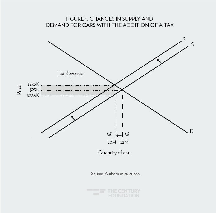
The top line shows the effective price to consumers, once the tax has been imposed. As a result of the tax, the price paid by consumers will be somewhat higher than it had been previously. However, the rise in car prices will also mean that consumers buy fewer cars. This means that car sellers will receive less money both because they are selling fewer cars, but also because the reduction in demand as a result of the tax will lead to a situation where they get less money per car. So the reduction in revenue to the auto industry will be the combined effect of selling fewer cars and getting less money for each car they sell.
The extent to which the before-tax price falls and the quantity is reduced depends on the relative shape of the supply and demand curves. (These curves are drawn in an arbitrary manner for purely illustrative purposes.) In this case, the tax of $5,000 per car is shown to be evenly shared between consumers and producers. The average price paid by a consumer rises from $25,000 without the tax to $27,500 with the tax. The average price received by auto manufacturers falls from $25,000 to $22,500. The gap of $5,000 per car is the tax revenue raised by the government.
This tax is associated with a drop in sales from 22 million to 20 million. The loss in revenue to manufacturers comes to $100 billion a year, the difference between selling 22 million cars at $25,000 each, or $550 billion, and selling 20 million cars at $22,500 each, or $450 billion. In this case, consumers are paying $2,500 more for each car they buy, but because they are buying 2 million fewer cars, their total spending on cars is unchanged at $550 billion.
In terms of assessing winners and losers, consumers clearly end up worse off to the extent that they valued the 2 million cars that they end up not purchasing as a result of the tax. Also, the consumers who do buy cars will have less money to spend on other items as a result of having to pay $2,500 more for each car they buy.
There will similarly be a burden imposed on car manufacturers. Since they are producing fewer cars, they will employ fewer workers and need a smaller amount of parts, materials, and capital equipment. This means fewer people will be employed both directly in the auto industry, and also indirectly in the various industries that produce inputs for the auto industry. The car manufacturers are also likely to see a reduction in profits due to the decline in both prices and sales.
The extent of the negative impact of the displaced workers will depend on their ability to get other jobs at comparable pay. If the pay at auto manufacturers and their suppliers is comparable to the pay in other sectors where these workers can find jobs, then the decline in car sales will have little impact on their standard of living once the adjustment process is completed. However, if the auto industry is a source of relatively high paying jobs for these workers, then the decline in sales would imply a reduction in their standard of living as they are forced to accept lower paying jobs in other sectors.
While the same sort of story would apply to any other industry that produced consumer goods or services, it is important to understand that the situation is notably different in an industry like finance that is primarily producing intermediate goods. Figure 2 shows the impact of a tax of $100 billion a year in the financial sector. (Again, these lines are drawn arbitrarily for illustrative purposes.)
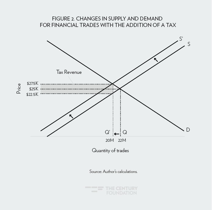
Figure 2 is drawn to show a decline in trading volume that is the same as the decline car volume shown in Figure 1, with the increase in the after-tax cost per trade equal to the increase in the after-tax cost of a car. (To be more realistic, these can be thought of as blocks of 1 million trades.) This leaves all the dollar sums the same as in Figure 1; however, the meaning on the consumer side is qualitatively different in a very important way.
In Figure 1, consumers saw a cost from the tax both because they paid more per car as a result of the tax, and also because they bought fewer cars. Cars are a consumption good, so the expectation is that if consumers ended up buying fewer cars as a result of the tax, they would be in some way worse off. By contrast, trading is not a good that directly provides value for consumers. Trading is only valued as a way to increase wealth. Any individual trade will have a winner and a loser, but these are offsetting. On average, investors are not made worse off by engaging in fewer trades.35
Figure 2 is drawn so that the decline in trading volume fully offsets the impact of the tax in raising the cost per trade to consumers. This means that consumers spend no more on trading, including the tax, than they did before the tax was put into place. In this scenario the consumer feels no direct impact of the tax. When we look at a tax on cars, the portion of the tax borne by consumers depends on the extent to which the price to consumers rises due to the tax. In the case of a tax on trading, there is no reason to care about the per-trade price, we care about the total amount spent on trading. If that does not increase, as shown in Figure 2, consumers will only see an impact from the tax if a lower volume of trading reduces the ability of the financial sector to serve the productive economy. (This issue will be addressed in the third section.)
This point is important. If an increased volume of trading does not lead to an increase in the efficiency of the productive economy, then consumers on aggregate cannot gain from the increased trades. There will be winners and losers on any individual trade, but in aggregate this would net out to zero. This means that many of the trades currently being undertaken by the people managing our 401(k)s, our IRAs, and our pension funds are wasteful. The people who undertake these trades earn money off of them, but on average, investors do not. In this case, if we can reduce the volume of trading, as would be the case with an FTT, we are saving investors and the economy money.
The impact of the tax from the standpoint of producers is unambiguous. It leads to both a reduction in trading volume and less money on each trade. This would imply that many fewer people will be employed in the industry and also that those who remain employed are likely to receive lower incomes. As noted in the example of a hypothetical tax in the auto industry, the impact on the displaced workers from the financial sector will depend on the difference between pay in the industry and pay in other sectors. Since the financial sector pays considerably more on average than other industries, displacement is likely to mean a substantial loss of income for workers in the financial sector, or at least the higher paid workers in the sector. (Displaced custodians and office assistants might not see much reduction in pay.)
The key point to be recognized is that, unlike a tax on other consumer items, a tax on the financial sector is generally not born borne directly by consumers. The immediate impact of the tax will be on suppliers of financial services; there will only be an impact on consumers if the downsizing of the industry reduces its ability to serve the productivity economy. If a smaller financial sector can serve the productive economy as well as a larger one, then the burden of the tax will be felt mostly or entirely by the industry.
The idea that a large financial sector might be a drag on growth has been supported by recent research from the Bank of International Settlements and the International Monetary Fund, which found an inverted U-shaped relationship between the size of the financial sector and the rate of growth of productivity.36 They found that for countries with under-developed financial sectors, a deeper financial sector was associated with more rapid growth. However, once the financial sector reached a certain level, further expansion relative to the size of the economy was associated with slower growth. This is consistent with the idea that the financial sector is pulling resources away from productive uses.
These analyses imply that people who could be employed productively in other sectors of the economy are doing tasks in the financial sector that provide little or no value. The excessive trading, which is the immediate focus of an FTT, would be one example of how resources could be wasted. However, the proliferation of complex financial instruments would be another aspect of the same problem. As noted in the first section, an FTT may make some types of financial instruments more costly and possibly eliminate the market for them altogether. If these instruments provide little benefit to the productive economy, then this would be another way in which the tax would make the financial sector more efficient.
Section III: The Implications of a Smaller Financial Sector
Liquidity, Trading Costs, and Interest Rates
The most immediate way in which higher transactions costs could affect the economy is through higher interest rates. The tax will reduce effective returns on assets, with the impact dependent on the volume of turnover. To take a simple case, if the before-tax return on an asset is 5.0 percent annually (net of other turnover costs) and the holding time is on average six months, a tax of 0.1 percent will reduce the return (holding turnover constant) by 4.0 percent.37 Of course, if the holding time increases more than in proportion to the tax, as implied by the assumption of a trading elasticity greater than 1.0, then the effect of the tax on returns is actually positive. As noted above, the total amount spent on trading is actually less as a result of the tax, which means other things equal, total returns would increase.
However, there can be a possibility that investors actually are willing to forego a substantial portion of their returns in exchange for increased liquidity. This would imply that interest rates are lower than would otherwise be the case precisely because investors have the option to trade frequently at low costs.
This impact could be substantial. For example, if there has been a reduction in average trading costs in the stock market of 0.5 percentage points over the last four decades (probably a low estimate of the actual reduction) and shares are traded on average twice a year, this would imply that the reduction in trading costs would be the equivalent of 20 percent of annual returns, using an assumption of 5.0 percent real returns. Comparable reductions in trading costs for bonds and other instruments would imply a similar impact on returns.
While this sort of impact cannot be ruled out a priori, few, if any, models of interest rate determination include transactions costs as a major factor. If trading costs did have a substantial impact on interest rates, we would expect real interest rates in the 1950s, 1960s, and 1970s to be far higher, other things equal, than they are today. Certainly there has been no obvious downward path for real interest rates in the United States and other countries as transactions costs have fallen.
One reason that there may not be a return premium corresponding to the change in average trading costs is that active traders are far from the typical investor. If most investors trade little, while a small minority trade a great deal, then average trading costs would have little relevance for most investors. In that case, a rise in transactions costs matters a great deal to active traders, but very little to more typical investors.
This is a factor with regard to the decision on whether to include government debt in the mix of assets subject to the tax. Burman suggests excluding government debt from the tax with the logic that any revenue derived from the tax will simply be offset by the higher interest rates that the government will have to pay on its debt. As noted above, it is not evident that changes in transactions costs are fully passed on in interest rates, but even assuming they are passed on, it does not follow that it would be desirable to exclude government debt from the tax.
Suppose that applying the tax to government debt would raise $30 billion annually (roughly the amount implied in the calculations above). The assumption of an elasticity of trading volume greater than 1.0 implies that trading costs will actually be reduced by an amount greater than $30 billion as a result of the tax. This reduction in trading volume corresponds to an actual reduction in resources used in the financial sector. Workers currently employed in the trading of government debt will instead be freed up to work in other areas. In fact, if we use the assumption in Burman of an elasticity of 1.25, then applying the tax to bond trades would have freed up more than $40 billion a year in resources for productive economic activity.
Under the assumption that the rise in interest rates fully offsets the impact of the tax on trading costs, the government will have no more revenue than if it had not taxed government debt. This means that the larger interest payments to bondholders would be roughly equal to the money it raised from applying the FTT to government debt. But these higher interest payments will now be supporting pension funds, 401(k)s, and other shareholders rather than financing the more rapid trading of bonds by the financial industry.
The only downside to the tax is that investors would know that their debt holdings would be somewhat less liquid. Again, this will matter more to the most active traders than the typical holder of government debt. In this scenario, the government effectively ends up increasing the resources available to the productive economy, while leaving its own revenue little changed, at the cost of somewhat lower liquidity in the market for government debt. An alternative way of posing the issue is that, in this example, the financial industry imposes a tax on the economy of $30 billion a year for the additional liquidity the markets provide on government bond sales compared to the liquidity provided in the 1990s. One can argue whether or not this additional liquidity would be worth this price, but it is important to be clear on the terms of the trade-off.
In addition to the question of liquidity, there is also an issue of whether the rise in transactions costs resulting from the tax would impair the ability of financial markets to allocate capital to its best uses. This would be an argument that higher transactions costs could lead to larger divergences between the market price of assets and their “true” price based on economic fundamentals, and that these divergences had measurable consequences for the allocation of capital. The first part of this argument is arguably true, but the question of the consequences is far from certain.
The first part depends on the impact of trading costs on volatility. There is fair bit of research on this topic. While the results are far from conclusive, a fair reading of the literature would probably support the view that lower trading costs are associated with reduced volatility.38 However, most of the research on the impact of trading costs and volatility is focused on short-term movements in asset prices, such as the average change in the price of a share of stock over the course of a day.
These short-term fluctuations in asset prices are really providing more information on the liquidity of markets than the ability of markets to direct capital to its best uses. If there are larger intra-day fluctuations in the price of stock or other assets, it increases the risk to an investor that they may buy the asset at a temporarily inflated price or sell at a temporarily depressed price (these deviations should average out, so on net the typical investor is neither helped nor hurt), but it is difficult to believe that it would have a measurable impact on the effective allocation of capital.
If a stock spends another hour or two 0.5 percentage points above or below its fundamental value (assuming that the market tends towards the fundamental value), it seems implausible that it would affect the flow of productive investment in a noticeable way. It seems unlikely that, except in the rarest of cases, such modest misalignments of prices would cause a company to undertake an investment it would not otherwise take or not to carry through an investment that would have been profitable. The same would apply to other assets like oil or corn. If the price of a barrel of oil is 0.5 percent higher than the fundamentals would imply for a few hours, it is difficult to envision a large amount of capital committed to drilling that would not be profitable at the price dictated by the fundamentals.
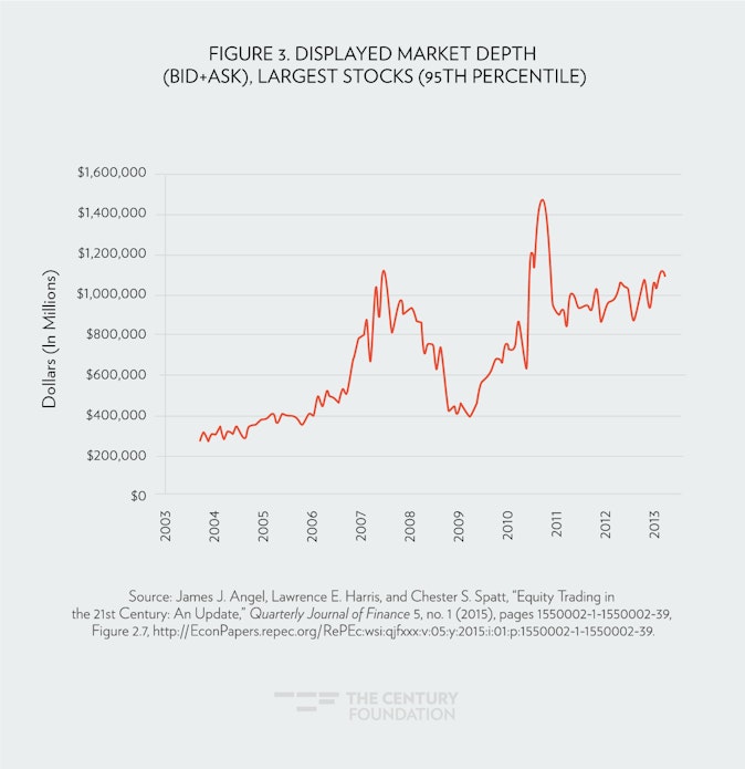
In this respect, even with a sharp reduction in trading volume, there is still likely to be far more liquidity in the market than existed just two decades ago. Figure 3 shows a measure of market depth, the average value of shares available to be bought or sold, since 2003. It shows that depth has more than tripled for the most highly traded stocks, indicating that if it fell by back by two-thirds, it would still be higher than it was in 2003. In other words, we are still likely to see more market depth in 2017 financial markets that have an FTT than in the 2003 market without an FTT.
While longer term and larger divergences between prices and fundamentals can affect the allocation of capital, the evidence in this area is far more uncertain. There have been several occasions in the last three decades where there were sharp movements in price that bore no obvious relationship to the fundamentals in the economy. The most obvious was the flash crash in 2010, which was due to a misreported price that triggered a sell-off by programmed trading. The main market indexes plunged by close to 10 percent over the course of 30 minutes. While this was reversed in a matter of hours, it is difficult to envision such swings being driven by human trading.
Similarly, no one ever found an explanation in market fundamentals for the crash in October 1987. This was also driven by program trading. It took close to two years to completely reverse this slide, although half of the loss was recovered in most markets within a week. It is not clear that the modest increase in trading costs associated with the sorts of FTTs being discussed would reduce the likelihood of large swings in prices caused by fluke events, but clearly these large swings would have more impact on the efficiency of markets in serving the productive economy than the modest deviations from fundamental values that may be associated with a decline in market volume and a corresponding reduction in liquidity. In other words, it is not clear that an FTT of the size being proposed here can have a sizable impact on destabilizing speculation. However, the fact that we have seen extraordinary and unexplained swings in prices in periods of low trading costs and high volumes suggests that reducing trading volume with an FTT is not likely to destabilize financial markets.
On the issue of the relationship between transactions costs and growth, modeling practices among macroeconomic forecasters generally do not assume that future growth will be faster as a result of declines in transaction costs in the financial sector. That practice may be mistaken, but modelers in the 1970s, 1980s, and 1990s, did not project an acceleration in growth rates in their forecasts as a result of predictable declines in transactions costs in financial markets.
While it has not led to faster economic growth, the explosion in the size of the financial sector since 1970 has been associated with an explosion in compensation in the industry. Compensation has always been higher in the financial sector than elsewhere in the economy, but in 1970 the gap was not nearly as large as it is now. In 1970, the average compensation for a full-time employee in the financial sector was less than 50 percent higher than the average for the economy as a whole. In 2014, compensation in the financial sector was almost 270 percent higher than the average for the economy as whole, as shown in Figure 4.39 Research has shown that as much as 18.4 percent of primary taxpayers in the top 0.1 percent of the income distribution are employed in finance.40
It is likely that the sort of downsizing of the industry that would be associated with a moderately sized FTT would lead to a substantial reduction in pay for many of the high earners in the financial sector. Many would undoubtedly move to other sectors, where their skills may still command a high wage, but likely less than they are currently earning in the financial sector. The workers who remained in the sector may still earn considerably more than the average for workers in other sectors, but the gap would almost certainly be less than it was before the tax. In effect, in order to maintain their share of shrinking market, workers in the financial sector would be forced to forego a substantial portion of their compensation.
Section IV: Using the FTT for Reducing or Eliminating College Tuition
In principle, tax revenue is fungible. Revenue raised from any source can be used for whatever purpose Congress designates. However, many proposals for an FTT have suggested designating the revenue for a specific purpose. Most notably, in his presidential campaign, Senator Bernie Sanders proposed using the revenue from an FTT to make public colleges tuition free. Financing college tuition is just one possible use of tax revenue. The projected $105.5 billion in revenue is almost fifteen times the projected annual cost of President Obama’s Preschool for All Initiative.41 It is also about 5 percent more than the current level of federal spending on infrastructure.42 It can be helpful, however, to hold up the Sanders’ example to get a better sense of the impact of the tax on the economy.
Sanders estimated the cost of his proposal for free college at $75 billion a year.43 This suggests that a financial transactions tax along the lines discussed in the prior section could easily cover the cost of free tuition. However, there will be important issues going forward. If the rate of growth of college costs continues to hugely outpace the overall rate of inflation, then at some point in the not distant future, the revenue from a financial transactions tax would not be sufficient to cover the cost. In addition, eliminating tuition at public colleges inevitably would also increase demand and thus enrollment at these schools.
Neither of these developments would necessarily be bad. One of the main points of the proposal is presumably to make college more accessible. And, achieving more socioeconomic integration in higher education (a very likely result of eliminating tuition at state schools) should generally be viewed as a positive development. Nonetheless, both outcomes will increase the cost of making public colleges free. If mechanisms are not put in place to restrict the growth of attendance and the cost of public higher education, then even the large sums that can be raised through a financial transaction tax will not be adequate.
However, there is an efficiency argument for free college that should be noted. There are very substantial costs associated with the sort of means-testing under the current system, in which tuition is high, but lower-income students are eligible for financial assistance. This requires a costly bureaucracy that has to review filing from students and their families. The situation is further complicated by the fact that many students come from families where parents are separated and one or both might seek to avoid any financial responsibility for their child’s college education. This can lead to situations where students are either assessed large tuition payments based on the income of a parent who is unwilling to support their education, or they are forced to spend a great deal of effort demonstrating this fact. Either situation is clearly unfortunate from the standpoint of trying to make college accessible to students regardless of their family background.
The other problem with even a generous system of financial aid is that many lower income students are likely to not recognize the potential benefits to them from such a system. One study found that less-educated and low-income parents often had little knowledge of the cost their children would face in attending college.44 They often overestimated the costs by a factor of two or three. This problem was especially prevalent among African American and Hispanic parents.
In principle, the lack of knowledge can be overcome by effectively providing information on financial aid to lower-income and minority parents, but this has not proven to be an easy task. Even with the most aggressive efforts at outreach, it is likely that many lower-income and minority students will still end up not attending college because they overestimate the costs they would face.
This would be a strong argument for making public colleges and universities tuition free. Replacing a complex system of financial aid with a simple system of free tuition would likely be the sort of change that would be widely recognized and understood. This should go far toward overcoming the information barrier that is preventing many otherwise qualified students from attending college.
However, even if we reject the goal of free college tuition, there is still a strong argument for increasing the public resources devoted to higher education. Attendance and graduation rates have risen very slowly in the past three decades among men. It is likely that the fear of incurring large debt, coupled with the large variance in earnings among graduates, has been a major factor.45 Furthermore, with many recent college graduates continuing to face a weak labor market, student debt from college loans is likely to be a substantial burden well into their careers. For these reasons, measures to reduce the cost of college offer large benefits for students from low- and-middle income families. And, of course, a more educated workforce will be a more productive workforce. By shifting resources from unproductive uses in the financial sector to education, we will be very directly increasing the productivity of the economy.
Conclusion
The evidence compiled in this report indicates that it should be possible to raise a substantial amount of revenue from an FTT, without disturbing the finance sector’s ability to serve the productive economy. Since there has been a sharp decline in the cost of transactions over the past four decades, even with a tax in place, transactions costs would still likely be lower than they were just two decades ago. This was a time the United States already had a robust financial market, so costs at this level should still be consistent with deep capital markets.
Furthermore, evidence on the elasticity of trading volume suggests that the reduction in volume will likely more than offset the increase in costs due to the tax for a typical trader. This means that most traders will actually see a reduction in total trading costs as a result of the implementation of an FTT. Instead, the burden of the tax will be borne by the financial sector, which is likely to become considerably smaller even in response to a modest sized FTT. There will only be a cost to households if the tax impeded the ability of the financial sector to efficiently allocate capital.
If the tax is dedicated to funding higher education, as some have suggested, this would amount to transferring resources from the financial sector to the education sector. This is likely to be a far more productive use of those resources.
Credits and Acknowledgements
This report was published by the Bernard L. Schwartz Rediscovering Government Initiative, founded in 2011 with one broad mission: countering the anti-government ideology that has grown to dominate political discourse in the past three decades.
Jeff Madrick is director of the Bernard L. Schwartz Rediscovering Government Initiative at The Century Foundation, where he is a senior fellow. He is a regular contributor to The New York Review of Books, and a former economics columnist for The New York Times. In addition to his work at The Century Foundation, Madrick also edits Challenge Magazine, and is a visiting professor of humanities at The Cooper Union. He is the author of numerous best-selling books on economics, and was a 2009 winner of the PEN Galbraith Non-fiction Award. Madrick was educated at New York University and at Harvard University, where he was a Shorenstein Fellow.
Notes
- Italy taxes over-the-counter stock transactions at a 0.2 percent rate.
- Robert Pollin, James Heintz, and Thomas Herndon, “The Revenue Potential of a Financial Transaction Tax for U.S. Financial Markets,” Political Economy Research Institute, 2016, http://www.peri.umass.edu/fileadmin/pdf/working_papers/working_papers_401-450/WP414.pdf.
- Stephan Schulmeister, Margit Schratzenstaller, and Oliver Picek, “A General Financial Transaction Tax: Motives, Revenues, Feasibility and Effects,” WIFO, March 2008, http://www.wifo.ac.at/jart/prj3/wifo/resources/person_dokument/person_dokument.jart?publikationsid=31819&mime_type=application/pdf.
- Leonard Burman et al., “Financial Transaction Taxes in Theory and Practice,” National Tax Journal, 69, no. 1 (March 2016): 171–216, http://www.brookings.edu/~/media/research/files/papers/2016/02/29-financial-transaction-taxes-in-theory-practice-gale/burman-et-al_-ntj-mar-2016-%282%29.pdf. More recently, the Tax Policy Center did an analysis of the Sanders plan and explained most of its differences with the PHH analysis (James R. Nunns, “A Comparison of TPC and the Pollin, Heintz and Herndon Revenue Estimates for Bernie Sanders’s Financial Transaction Tax Proposal,” Tax Policy Center, April 12, 2016, http://www.taxpolicycenter.org/sites/default/files/alfresco/publication-pdfs/2000738-A-Comparison-of-TPC-and-the-Pollin-Heintz-and-Herndon-Revenue-Estimates-for-Bernie-Sanders-Financial-Transaction-Tax-Proposal.pdf). This analysis put the revenue from a Sanders-type tax at $52 billion, slightly higher than their earlier calculation. The discussion in this study focuses on the fuller analysis in Burman et al., but little would be changed by addressing the Nunns analysis.
- Japan Securities Research Institute, “Securities Market in Japan,” Japan Securities Research Institute, 1992, 244.
- Securities and Exchange Commission, “Fee Rate Advisory #3 for Fiscal Year 2016,” January 7, 2016, https://www.sec.gov/news/pressrelease/2016-2.html.
- Thornton Matheson, “Security transaction taxes: issues and evidence,” International Tax and Public Finance 19, no. 6 (2012): 884–912.
- he tax applies to derivatives on stock, but only if they are exercised. This would exclude the overwhelming majority of derivate transactions.
- This calculation uses data from Inland Revenue Service, “Assessment and collection of stamp duty,” in Director of Audit’s Report no. 54, Chapter 2, Table 1 (Hong Kong: Audit Commission, March 29, 2010), http://www.aud.gov.hk/pdf_e/e54ch02.pdf.
- he figure in the table for Japan for 1990 contradicts other evidence. The Japan Securities Research Institute (1992) put the revenue raised from the Japanese financial tax in that year (the peak of the stock bubble) at 1.1 percent of GDP.
- Robert Pollin et al. proposed a rate structure that was intended to double current transactions costs, so as not to bias the tax against specific instruments. (Robert Pollin et al., “Security Transactions Taxes for U.S. Financial Markets,” Eastern Economic Review 29, no. 4 [2003]: 527–58, http://www.peri.umass.edu/236/hash/aef97d8d65/publication/172/.) This, of course, requires knowledge of what current transactions costs are.
- The SIFMA data are available at http://www.sifma.org/uploadedFiles/Research/Statistics/StatisticsFiles/CM-US-Equity-SIFMA.xls?n=53461.
- Dean Baker et al., “The Potential Revenue from Financial Transactions Taxes,” Center for Economic and Policy Research, 2009, http://cepr.net/documents/publications/ftt-revenue-2009-12.pdf.
- Bank for International Settlements, “Derivative Statistics,” BIS, 2015, http://www.bis.org/statistics/extderiv.htm.
- Bank for International Settlements, “Derivative Statistics,” BIS, 2015, http://www.bis.org/statistics/about_derivatives_stats.htm.
- Bank for International Settlements, “Derivative Statistics,” BIS, 2015, http://www.bis.org/statistics/derstats3y.htm.
- The 2013 data are adjusted up by 10 percent for growth between 2013 and 2015, but then reduced by 10 percent under the assumption that U.S. trades account for 90 percent of North American trades, which is the category given by BIS. This figure is similar to the one calculated in Nunns, “A Comparison of TPC. . . .”
- Nunns, “A Comparison of TPC . . .” uses the same higher equity transactions volume as PHH.
- Schulmeister, Schratzenstaller, and Picek, “A General Financial Transaction Tax.”
- This figure is obtained by calculating the response of revenue to changes in the size of the tax.
- Bureau of Economic Analysis, “National Income and Product Accounts Tables,” retrieved May 10, 2016, from http://www.bea.gov/national/Index.htm.
- This figure would not include intermediate inputs, like the use of electricity and other utilities and supplies of paper, but these are almost certainly of little consequence in this sector. On the other side, not all the income in this sector stems from trading. The firms in this sector derive substantial revenue from underwriting new issues and also from management fees not directly associated with trading. The amount of income derived from trading would almost certainly be considerably less than the total income calculated for the industry.
- Michael Fleming, “The Round-the-Clock Market for U.S. Treasury Securities,” FRBNY Economic Policy Review, July 1997, https://www.newyorkfed.org/medialibrary/media/research/epr/97v03n2/9707flem.pdf.
- In this respect, it is worth noting that Schulmesieter et al. report trading costs for S&P 500 index contracts of just 0.0016 percent of the nominal value and for three-month interest contracts in Eurodollars of 0.0006 percent (Schulmeister, Schratzenstaller, and Picek, “A General Financial Transaction Tax,” Table A-4). This is consistent with the view that the most widely traded assets are generally traded at extremely low costs.
- Thornton Matheson, “Taxing Financial Transactions: Issues and Evidence,” IMF Working Paper WP/11/54, 2011, https://www.imf.org/external/pubs/ft/wp/2011/wp1154.pdf.
- One of the reasons that the response of trading volume was so small is that these taxes have raised relatively little revenue to date. The tax in France only raised 700 million euros in 2015. Adjusting for GDP, this would be the equivalent of roughly $4 billion in the United States (Cécile Barbière, “French plans to expand FTT may sink European negotiations,” EurActiv, October 12, 2015, http://www.euractiv.com/section/development-policy/news/french-plans-to-expand-ftt-may-sink-european-negotiations/). It should not be surprising that a tax that has raised little revenue would have little effect on trading volume.
- Since trading is an intermediate good (it does not directly provide a benefit to consumers), there is not an issue about it being a luxury good, the relative demand for which increases as income rises. (An exception would be if trading is actually a form of gambling that people do value as an end in itself. If this is the case, then an FTT would take the form of a sin tax, discouraging people from engaging in potentially harmful behavior.)
- Robert Pollin et al., “Security Transactions Taxes for U.S. Financial Markets,” Eastern Economic Review 29, no. 4 (2003): 527–58, http://www.peri.umass.edu/236/hash/aef97d8d65/publication/172/.
- Burman et al. note the trend of declining transactions costs. Their calculations assume that transactions cost fall by 50 percent from 2010 to 2035. Matheson (“Taxing Financial Transactions”) notes that bid-ask spreads on the NYSE have fallen more than 90 percent since the mid-1980s.
- A fuller discussion of design issues can be found in Pollin et al., “Security Transactions Taxes for U.S. Financial Markets.”
- Note that this is not a revenue maximizing tax rate. The revenue maximizing rate would be 0.8 percent on stocks, assuming an elasticity of -1.25. While it may prove desirable to move to a revenue maximizing rate, it would probably not be advisable to introduce the tax at such a high rate. If the tax proved not to lead to major market disruptions, then it should be possible to raise the rate after it was implemented.
- Burman et al. lowered their revenue estimate by $29 billion to account for lower taxable income as a result of the tax. The extent to which the tax leads to a reduction in taxable income would depend on the extent to which a rise in transactions costs affect the economy, which is the topic of the next section. Most immediately, the tax does not reduce the income of investors, as the tax payments are more than fully offset by reductions in trading costs.
- The size of the sector was calculated from Bureau of Economic Analysis data by taking the lines for compensation in the securities and commodities trading industry and also investment funds and trusts (Bureau of Economic Analysis, “National Income and Product Accounts Tables,” Table 6.2D, lines 59 and 61 for 2014 and Table 6.2B, lines 55 and 59 for 1970). The calculation attributes income in the financial sector from proprietorships (Table 6.12D, Line 14 for 2014 and Table 6.14D, Line 14 for 1970) and corporate profits (Table 6.16D, Line 12 for 2014 and 6.16B, Line 12 for 1970) in proportion to the narrower trading sector’s share of employee compensation to employee compensation in the financial industry as a whole.
- Employment in the securities and commodities trading sector was a bit less than 900,000 in 2014 (Bureau of Economic Analysis, “National Income and Product Accounts,” Table 6.4D, Line 49).
- There is a possibility that some people do view trading as a form of recreation like casino gambling. This discussion assumes that the bulk of trading is not done for recreational purposes.
- Stephen G. Cecchetti and Enisse Kharroubi, “Reassessing the impact of finance on growth,” Bank of International Settlements, BIS Working Papers no 381, July 2012, http://www.bis.org/publ/work381.pdf; Ratna Sahay et al., “Rethinking Financial Deepening: Stability and Growth in Emerging Markets,” International Monetary Fund, IMF Staff Discussion Note, May 2015, http://www.imf.org/external/pubs/ft/sdn/2015/sdn1508.pdf.
- Burman et al. includes a useful table (Table 3) showing the impact of tax rates on the rate of return for different holding periods.
- Matheson (“Taxing Financial Transactions”) has a good summary of the research on the relationship between trading costs and volatility.
- These figures are obtained from Bureau of Economic Analysis by dividing total employee compensation (Bureau of Economic Analysis, “National Income and Product Accounts,” Table 6.2B, lines 55 and 59, and Table 6.2D, lines 59 and 61) by the number of full-time equivalent workers in the sector (Table 6.5B, Line 55, and Table 6.5D, line 59).
- J. Bakija, A. Cole, and B. Heim, “Jobs and Income Growth of Top Earners and the Causes of Changing Income Inequality: Evidence from U.S. Tax Return Data,” Manuscript, Williams College, 2012.
- U.S. Department of Education, “Initiatives: Early Learning,” retrieved May 31, 2016, http://www2.ed.gov/about/inits/ed/earlylearning/index.html.
- Congressional Budget Office, “Public Spending on Transportation and Water Infrastructure, 1956 to 2014,” 2015, https://www.cbo.gov/publication/49910.
- Even conservative critics have agreed that this figure is a reasonable estimate of the cost of the proposal (see, for example, James Pethokoukis, “How much will ‘free college’ cost? New study suggests colleges respond to more financial aid by increasing tuition,” American Enterprise Institute, 2016, http://www.aei.org/publication/how-much-will-free-college-cost-new-study-suggests-colleges-respond-to-more-financial-aid-by-increasing-tuition/).
- Eric Grodsky and Melanie T. Jones, “Real and imagined barriers to college entry: Perceptions of cost,” Social Science Research 36, no. 2 (June 2007): 745–66.
- John Schmitt and Heather Boushey, “The College Conundrum: Why the Benefits of a College Education May Not Be So Clear, Especially to Men,” Center for American Progress, 2010, https://www.americanprogress.org/wp-content/uploads/issues/2010/12/pdf/college_conundrum.pdf.